11 Lesson 11
11.1 Building Memex - Step 5
- Searching our publications
- Extra: visualizong tf-idf terms with wordclouds
- Extra+: a function for loading stopwords
11.2 Running searches
As we discussed today, we are likely to lose some information because of imperfect OCR results, although it is hard to tell to what extent that affects connections that we generate using tf-idf values (a way to test this would be to compare connections generated for text files of high quality and artificially generated OCR results for these very text files). In any case, connections that we generated are not a substitute for searches, rather they complement each other increasing the overall value of our memex.
What would we want? The general idea is that we want to search all our OCRed publications, present results in a convenient manner that would allow us to go directly to specific publications. In practical terms that would mean that we want to write a function that:
- takes a search string as one of its arguments (other arguments are up to you); we can and should use regular expressions here;
- loads data on all files with OCR results;
- loops through these files (since we saved OCR results as dictionaries of page numbers and page contents, we can loop through all the pages and check if they contain what we are looking for);
- collects pages with matches into a dictionary of search results;
- we can use the same dictionary-of-dictionaries structure that we have already used before;
- the dictionary will have citeKeys as its
keys, and the dictionary of matches for itsvalues; - the dictionary of matches will have page numbers as its
keysand search matches as itsvalues; for search matches we may also want additional information, such as number of matches on a page; a link to the original (html) page within our memex (although this can also be generated later, when we update the interface). - for the main dictionary with the results we may also want to save additional information for the entire search, like the date and time (timestamp) of our search and the exact string we have been using for searching.
Overall the results should look like the example below (I have manually shortened result values for better view):
{
    "000000009::::GrazierHollyweird2015": {
        "0253": {
            "matches": 2,
            "pathToPage": "g/gr/GrazierHollyweird2015/pages/0253.html",
            "result": "...being to describe the collection of all potential
            universes—the most com-<br>mon of which is <span class='searchResult'>
            multiverse</span>.<br><br>There are many of us thinking of one version
            of parallel universe theory or an-<br>other. If it’s all a lot of
            nonsense, then it’s a lot of ... If there are parallel universes,
            would we ever be able to detect them? Travel<br>to them? For some
            <span class='searchResult'>multiverse</span> models, the surprising answer is..."
        },
        "0260": {
            "matches": 4,
            "pathToPage": "g/gr/GrazierHollyweird2015/pages/0260.html",
            "result": "...The quantum <span class='searchResult'>multiverse</span>
            is an outcome of the Many Worlds interpretation<br>of quantum mechanics,
            proposed by Hugh Everett in 1957. The many-worlds<br>hypothesis is an
            attempt to solve a very deep problem in quantum mechanics,<br>the
            Schrédinger’s Cat problem. Recall that for the Schrédinger’s Cat gedanken<br>
            experiment, imagine a cat sealed in a box, with a 50-50 chance of living
            or<br>dying in a given time period T. After time T elapses, what can
            we say about<br>the cat? Nothing. ...<br>"
        },
    },
    "000000009::::GribbinErwin2012": {
        "0294": {
            "matches": 2,
            "pathToPage": "g/gr/GribbinErwin2012/pages/0294.html",
            "result": "... The <span class='searchResult'>Multiverse</span> idea says
            that there always were<br>256 universes, identical to one another up to
            the point where<br>the computation is run, and that the identical
            experimenters<br>in each of those universes each decide to carry
            out the same<br>experiment—hardly surprising, since they are identical..."
        }
    },
    "searchString": "multi\\W*verse",
    "timestamp": "2021-01-12 15:32:11"
}
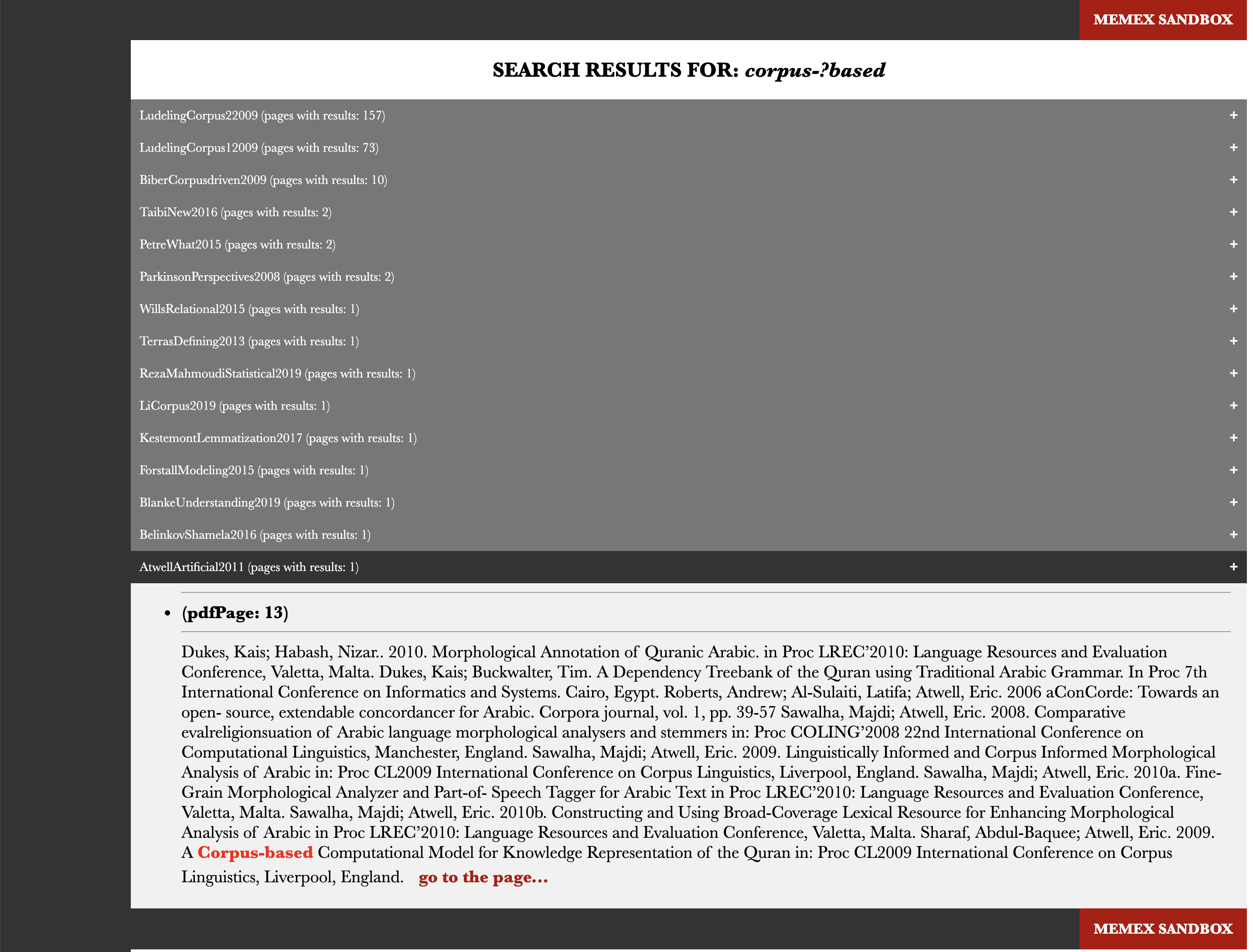
After we have search results collected and saved, we would, of course, want to make them easily available. We would want to be able to preview those results (to see the match in context) and to go to the original page. Your page may look something like on the screenshot below, where 1) results are grouped by publications and ranked by the number of matches per publication; 2) clicking on the citeKey of a publication opens the preview with matches and you can click on a link to get to the original HTML page:

To simplify the task of generating such an html page with results, you can use this html code as your guide and template.
Remember that you can always adjust the code to fit your own goals. As we briefly discussed, you can add a function that would run some normalization (or, rather, de-normalization) of your search strings to catch words that might have been recognized with errors during the OCR process. For example, if you are searching for Schrödinger (and not his cat :), you need to modify your search string in such a way that we can find this word with its most common misspelling (if you looked carefully at the example above, you would have noticed that the name of this physicist was misspelled as Schrédinger). The following automatic modification will help to create a regular expression that will catch the most common misspelled forms (Schrédinger, Schrodinger, Schriidinger, etc.). You can easily write a function that will apply such modifications to all problematic letters.
11.3 Wordclouds as visual summaries
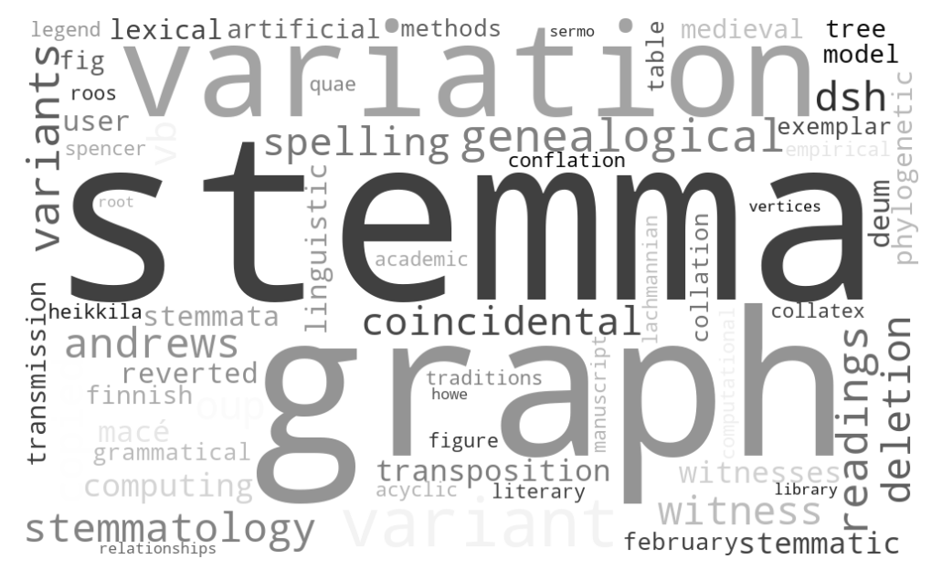
Wordsclouds can be a rather nice way to graphically represent keywords of publications. They can be problematic as more often than not they are created to be a pretty picture rather than an informative visualization (we can discuss this issue later). Be that as it may, wordclouds can add a nice touch to our project. Let’s create them.
The following code will generate a wordcloud if you provide the function with the path to save file and a dictionary of tf-idf terms:
from wordcloud import WordCloud
import matplotlib.pyplot as plt

AndrewsTree2013 = {
        "academic": 0.05813626462255791, "acyclic": 0.06250123247317078,
        "andrews": 0.12638860902474044, "artificial": 0.07179606130684399,
        "coincidental": 0.107968929904822, "collatex": 0.05992322690922588,
        "collation": 0.06303029408091644, "computational": 0.05722784996783764,
        "computing": 0.10647437138201694, "conflation": 0.06207493202469115,
        "copied": 0.11909333470623461, "deletion": 0.1139260485820703,
        "deum": 0.08733065096290674, "dsh": 0.12062758085160386,
        "empirical": 0.06256016440693514, "exemplar": 0.06413026390502427,
        "february": 0.06598308140156786, "fig": 0.06658631708313895,
        "figure": 0.057484475246214396, "finnish": 0.06718916017623287,
        "genealogical": 0.14922848147612744, "grammatical": 0.06639003369358097,
        "graph": 0.3064885690820798, "heikkila": 0.06250123247317078,
        "howe": 0.0502983742283863, "lachmannian": 0.05357248497700353,
        "legend": 0.05576734763473662, "lexical": 0.07504108167413616,
        "library": 0.052654345617120235, "linguistic": 0.08295373338961148,
        "literary": 0.05453901405048022, "macé": 0.09416507085735495,
        "manuscript": 0.056407679242811995, "medieval": 0.0722276960100237,
        "methods": 0.06617794961055612, "model": 0.06712481163842804,
        "oup": 0.11328056728336285, "phylogenetic": 0.0771729868291211,
        "quae": 0.06207493202469115, "readings": 0.14004936139939653,
        "relationships": 0.05294605101492676, "reverted": 0.08384604576952619,
        "roos": 0.057864729221843304, "root": 0.050044699046501814,
        "sermo": 0.05136276592219361, "spelling": 0.10943421974916011,
        "spencer": 0.058047262455825824, "stemma": 0.42250289612460745,
        "stemmata": 0.0813887983497219, "stemmatic": 0.09093028877718234,
        "stemmatology": 0.11984645381845176, "table": 0.0650730361130049,
        "traditions": 0.06135920913100084, "transmission": 0.07196157976331963,
        "transposition": 0.09182278547380966, "tree": 0.06790095059625004,
        "user": 0.08246083727188196, "variant": 0.2562367460915465,
        "variants": 0.1432698250058143, "variation": 0.2935924450487041,
        "vb": 0.11035543471056206, "vertices": 0.050436368099886865,
        "vienna": 0.07506704856975273, "witness": 0.11471933221048437,
        "witnesses": 0.09101116903971758
    }

savePath = "AndrewsTree2013.jpg"

def createWordCloud(savePath, tfIdfDic):
    wc = WordCloud(width=1000, height=600, background_color="white", random_state=2,
                   relative_scaling=0.5, colormap="gray")
    wc.generate_from_frequencies(tfIdfDic)
    # plotting
    plt.imshow(wc, interpolation="bilinear")
    plt.axis("off")
    #plt.show() # this line will show the plot
    plt.savefig(savePath, dpi=200, bbox_inches='tight')

createWordCloud(savePath, AndrewsTree2013)
The result will look something like this:

Hint: you can always use the file with tf-idf values that you generated before, although you might want to change max_df and min_df parameters for wordclouds (for example, min_df=1 and max_df=0.75).
One more thing: experiment with how your wordclouds look. You can find lot of different parameters in the official documentation of the library — you can change colors, fonts, shapes, sizes, etc.
11.4 Stopwords for tf-idf
I have added a function for loading lists of stopwords. You can find it in functions.py.
11.5 Homework
- described above;
- additionally, take the solution scripts from the previous lesson and annotate every line of code; submit your annotations together with the main assignment; if you have any suggestions for improvements, please share them (this will count as extra points :).
- upload your results to your memex github repository
- place annotated scripts into
_miscsubfolder
- place annotated scripts into
11.6 Homework Solution
the working scripts have been added to the main repository on github