10 L10: GIS IV

10.1 Mapping Networks

10.2 Goals

• Basic understanding of networks
• Data for networks: nodes and edges
• Modeling networks
• Most common approaches

10.3 Software

• R, RStudio
  • igraph and a few other new libraries
    • NB: igraph is the main SNA library. There are other packages we can use to visualize graphs (ggraph, for example), but most calculations and the overall analysis is still to be performed with igraph. You can get an overview of its contents with library(help="igraph"). More information: https://igraph.org/r/; full documentation: https://igraph.org/r/doc/igraph.pdf
• Data:
  • Our practice datasets will include two data sets on Islamic history: 1) the route network of the islamic world around 9-10th centuries (https://althurayya.github.io/); and bio-geographical data collected from 30,000 medieval biographies (Source: “The History of Islam” (Taʾrīḫ al-islām) of al-Ḏahabī (748/1348 CE)): Islamic_World_Data.zip

# General ones 
library(tidyverse)
library(readr)
library(stringr)
library(ggplot2)

# SNA Specific
library(igraph)
library(ggraph)
library(ggrepel)
library(ggalt)

# mapping
library(rnaturalearth)
library(rnaturalearthdata)
library(grid) # grid library cuts out the plot from the graph

10.4 Networks (Graphs)

10.4.1 Basic Concepts and Ideas

10.4.1.1 Nodes (Vertices, Points)

graphObject <- graph_from_literal(
  1, 2, 3, 4, 5, 6, 7, 8, 9, 10, 11, 12,
  13, 14, 15, 16, 17, 18, 19, 20, 21, 22, 23)

set.seed(5)
plot(graphObject)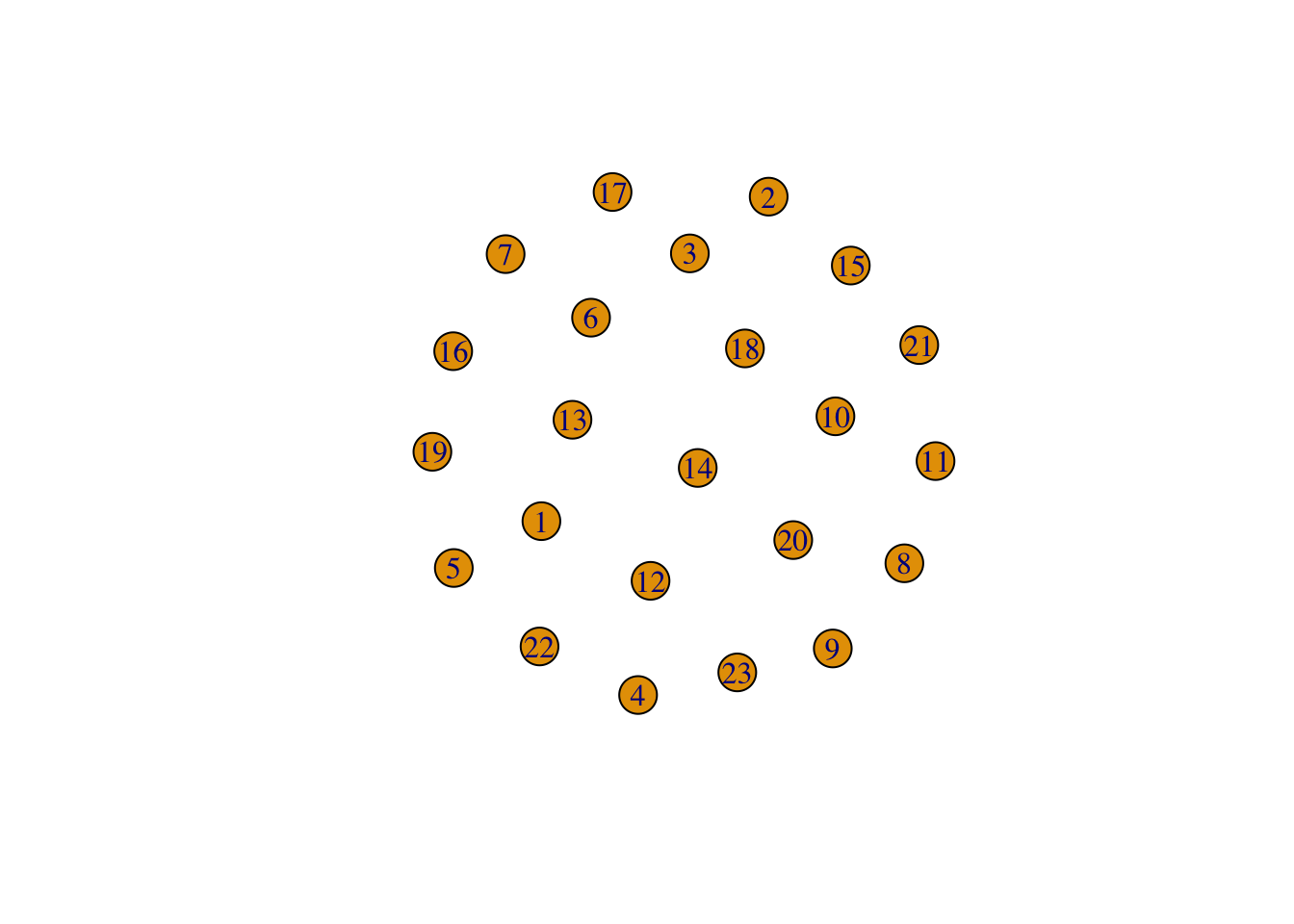

10.4.1.2 Edges (Links)

graphObject <- graph_from_literal(
  1--2:3:4:6:7:8:9, 2--1:20:22:11:3, 3, 4, 5, 6, 7, 8, 9, 10, 11, 12,
  13, 14, 15, 16, 17, 18, 19, 20, 21, 22, 23)

set.seed(5)
plot(graphObject)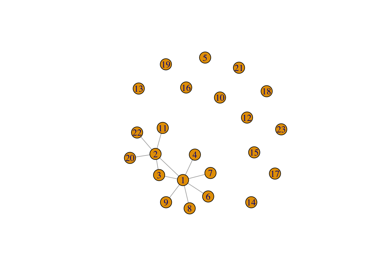

graphObject <- graph_from_literal(
  1--2:3:4:6:7:8:9, 2--1:20:22:11:3, 3--1:2:11:10:4, 4--1:3:10:5:6,
  5--6:4:10:12:6, 6--1:4:5:12:15,6-7, 7--1:6:15:16:8, 8--1:7:16:17:9,
  9--1:8:17:19:20, 10--3:11:23:12:5:4, 11--2:22:10:3, 12--5:10:23:13:15:6,
  13--12:23:14:15, 14--13:17:16:15, 15--6:12:13:14:16:7, 16--7:15:14:17:8,
  17--14:18:9:8:16, 18--9:17:19, 19--9:18:21:20, 20--2:9:19:21,
  22--2:20:21:11, 23--10:13:12)

set.seed(5)
plot(graphObject)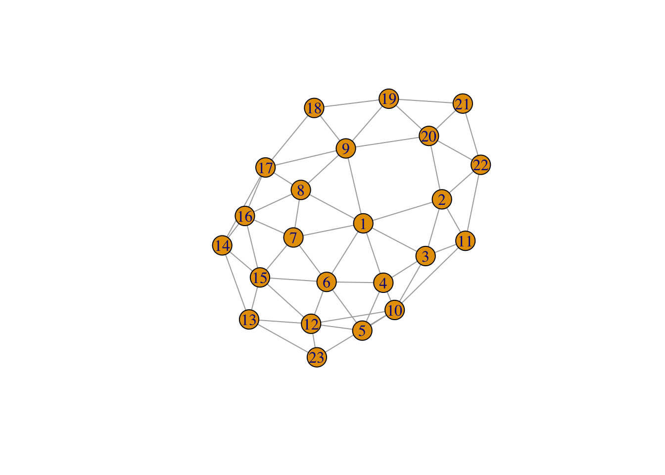

10.4.1.3 Major measures

# centrality measures
V(graphObject)$degree <- degree(graphObject, mode="all")
V(graphObject)$centr_degree <- centr_degree(graphObject, mode="all", normalized=T)$res

V(graphObject)$centr_eigen <- centr_eigen(graphObject, directed=F, normalized=F)$vector

V(graphObject)$betweenness <- betweenness(graphObject, directed=F)
V(graphObject)$centr_betw <- centr_betw(graphObject, directed=F, normalized=T)$res

# clustering (selected algorithms) some of these alrgorithms may take a while to run on large graphs
V(graphObject)$cl_walktrap <- as.character(cluster_walktrap(graphObject)$membership)
V(graphObject)$cl_louvain <- as.character(cluster_louvain(graphObject)$membership)

test <- as_data_frame(graphObject, what="vertices")

10.4.1.4 Degree centrality:

set.seed(5)

ggraph(graphObject, 'igraph', algorithm = 'with_fr') +
  geom_edge_link(width=0.5) +
  geom_node_point(aes(size=degree, color=degree), alpha=1) +
  geom_node_label(aes(label=name), color="black", size=3, repel=TRUE, alpha=1) +
  ggforce::theme_no_axes() +
  theme_graph() +
  scale_colour_gradient(low="black", high="red") +
  scale_size_continuous(range=c(1,10))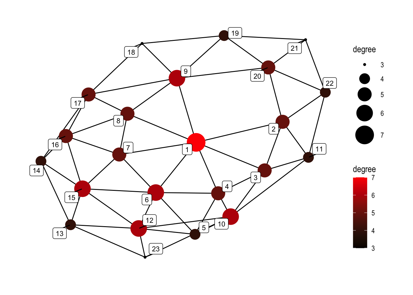

10.4.1.5 Betweenness / Betweenness centrality:

set.seed(5)

ggraph(graphObject, 'igraph', algorithm = 'with_fr') +
  geom_edge_link(width=0.5) +
  geom_node_point(aes(size=betweenness, color=betweenness), alpha=1) +
  geom_node_label(aes(label=name), color="black", size=3, repel=TRUE, alpha=1) +
  ggforce::theme_no_axes() +
  theme_graph() +
  scale_colour_gradient(low="black", high="red") +
  scale_size_continuous(range=c(1,10))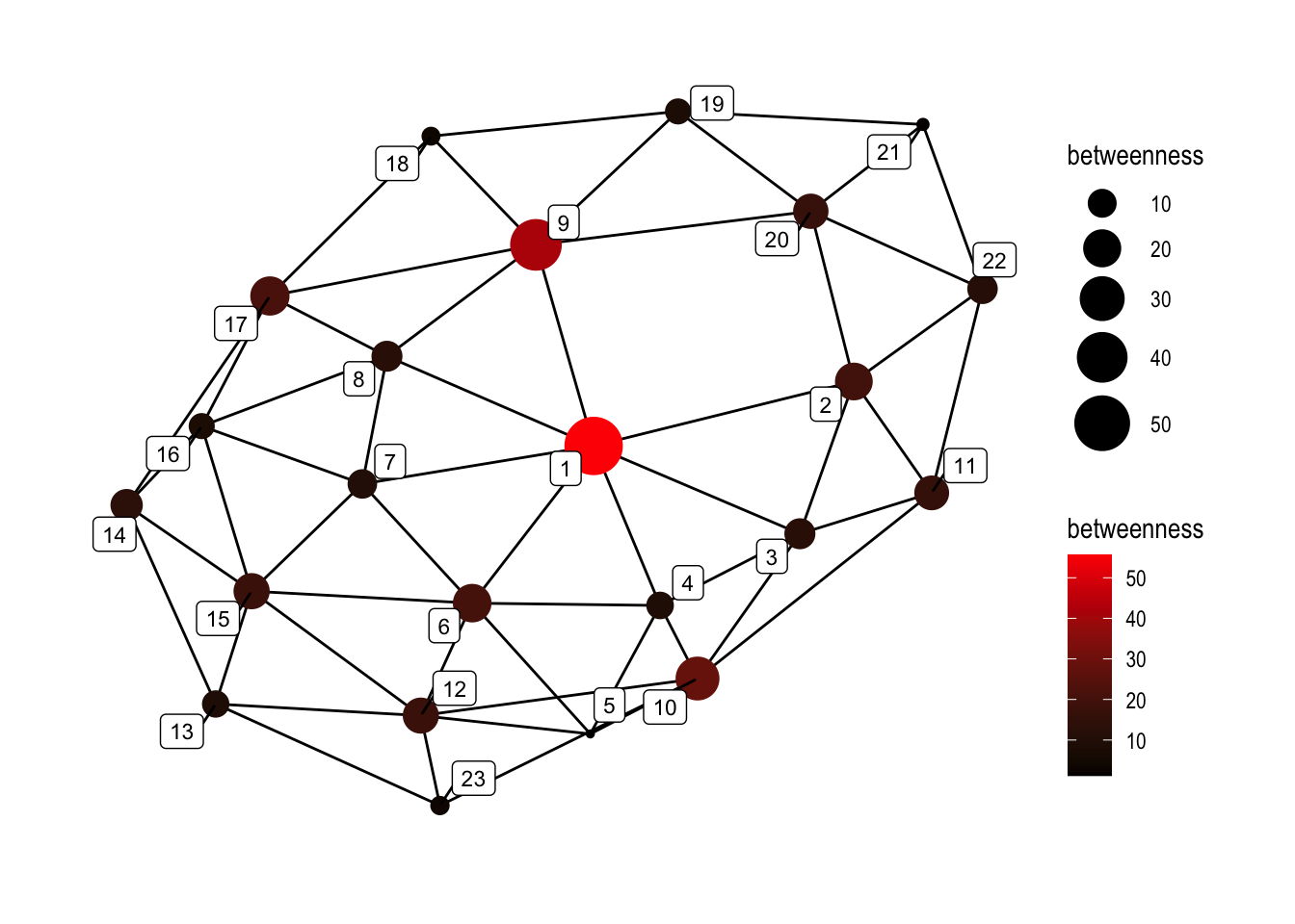

10.4.1.6 Eigenvector centrality:

set.seed(5)

ggraph(graphObject, 'igraph', algorithm = 'with_fr') +
  geom_edge_link(width=0.5) +
  geom_node_point(aes(size=centr_eigen, color=centr_eigen), alpha=1) +
  geom_node_label(aes(label=name), color="black", size=3, repel=TRUE, alpha=1) +
  ggforce::theme_no_axes() +
  theme_graph() +
  scale_colour_gradient(low="black", high="red") +
  scale_size_continuous(range=c(1,10))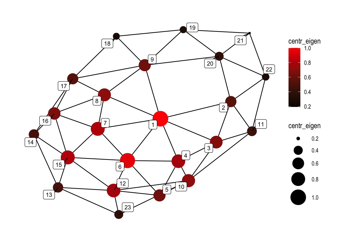

10.4.1.7 Clustering/Communities:

set.seed(5)

ggraph(graphObject, 'igraph', algorithm = 'with_fr') +
  geom_edge_link(width=0.5) +
  geom_encircle(s_shape=.1, expand=0.01, alpha=.25, col="black", aes(x=x, y=y, group=cl_louvain, fill=cl_louvain))+
  geom_node_point(aes(color=cl_louvain, size=degree), alpha=1) +
  geom_node_label(aes(label=name), color="black", size=3, repel=TRUE, alpha=1) +
  ggforce::theme_no_axes() +
  theme_graph()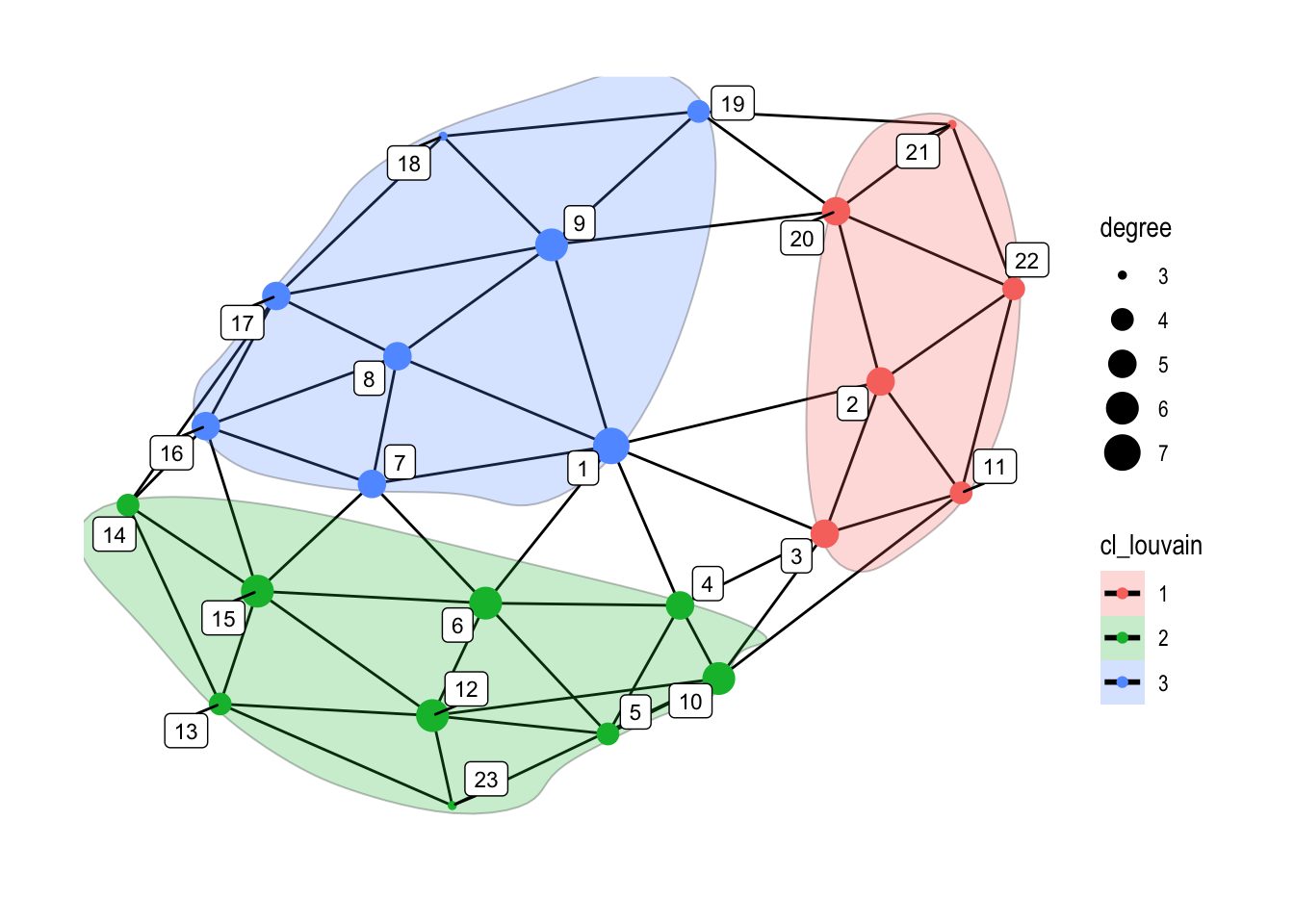

set.seed(5)

ggraph(graphObject, 'igraph', algorithm = 'with_fr') +
  geom_edge_link(width=0.5) +
  geom_encircle(s_shape=.1, expand=0.01, alpha=.25, col="black", aes(x=x, y=y, group=cl_walktrap, fill=cl_walktrap))+
  geom_node_point(aes(color=cl_walktrap, size=degree), alpha=1) +
  geom_node_label(aes(label=name), color="black", size=3, repel=TRUE, alpha=1) +
  ggforce::theme_no_axes() +
  theme_graph()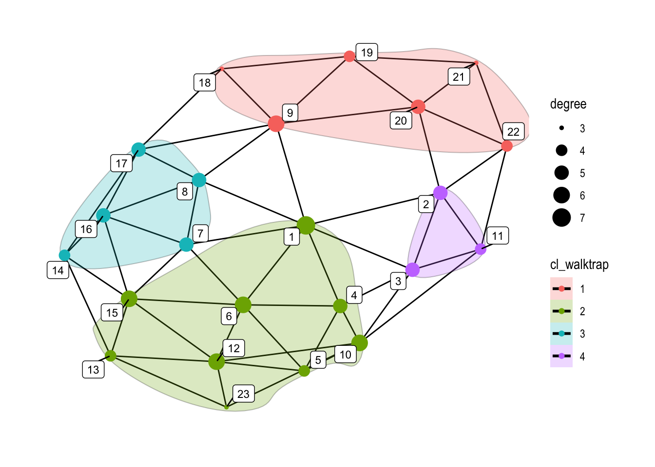

10.4.2 Data for Networks: Nodes and Edges

10.4.3 Modeling a Network

Hypothetical example: people with different political views living in Vienna.¹

• Data (tabular): person, residence district, frequented districts, dates (1800-2000), political views;
• Possible Networks:
  • Option 1: nodes: persons; edges: residence districts (this one will not be a geographical network); edges weights: no weights;
  • Option 2: nodes: districts; edges: people (edges between the residence district and frequented districts: 1–2, 2–3, 1–3); edges weights: the number of same edges;
  • Option 3: nodes: districts; edges: political views (edges between the residence district and frequented districts of people with shared political views: 1–2, 2–3, 1–3); edges weights: the number of same edges;
  • Option 4: and so on…

A note on unimodal (only one types of nodes), bimodal, and multimodal networks:

Image source: https://scottbot.net/lets-talk-about-networks/.

Nodes: authors and their books; Edges: authorship

Nodes: authors and their books; Edges: authorship, collaboration

Main points:

• one should always find ways to convert data into unimodal networks, as this is the type of networks that most algorithms are designed to work with;
• a bimodal network should be converted into a unimodal network (or, perhaps, a series of unimodal networks) where the second type of nodes becomes edges and their weights.
• for example: a bimodal network: nodes are individuals and cities, edges—connections of individuals to cities; connections of cities to cities; connections of individuals to individuals (potentially); unimodal networks: nodes are individuals; edges are shared cities with which individuals are connected. Thus, in this case, a connection between two individuals become the city that they havein common; the weight of this connection may be based on a number of shared cities. In other words, the connection between two individuals that share ten same cities will be stronger than between individuals that share only one; and there will be no connection between individuals who have no cities in common.
• unimodal network: one type of nodes; one type of connections; that said, the weight of connections may be aggregated from multiple parameters. For example, we have three individuals who share the city of Vienna as their connection; however, person 1 and person 2 also share something else—a district; the period of their lives overlap, etc., while person 1 and person 3 lived in different districts and their lives did not overlap chronologically. Thus, the weight of the edge between person 1 and 2 will be larger, than between 1 and 3 and two and 3. Yet, if there is also person 4, who has no connection to Vienna, his/her connection to P1, P2, and P3 will be nonexistent, unless we consider other parameters for the edges (shared lifetime, for example; or, larger geographical entities, etc.)

10.4.4 Most common analytical procedures: some recipes

10.4.4.1 Basemap

Download this file with extra data layers: map_objects.zip. Unzip it and make sure to change the path in the code below so that you can load the data.

RDSfolder="./data_temp/map_objects/"

rivers_df <- readRDS(paste0(RDSfolder,"rivers_df.rds"))
aral_sea_df <- readRDS(paste0(RDSfolder,"aral_sea_df.rds"))
routes_df <- readRDS(paste0(RDSfolder,"routes_df.rds"))

Now, le’t create a base layer map, as we did before:

NB: to install rnaturalearthhires, you may need to run: remotes::install_github("ropensci/rnaturalearthhires")

Base layer for the medieval Islamic world:

world <- ne_countries(scale="medium", returnclass="sf")

colWater= "lightsteelblue2"
colLand = "white"
colRout = "grey"

#xlimVal=c(-12,80); ylimVal=c(10,50)
IslamicWorldBaseBare <- ggplot(data=world) +
  geom_sf(fill=colLand, color=colLand) +
  # rivers, aral sea, and routes
  geom_path(data=routes_df, aes(x=long, y=lat, group=id), color=colRout, size=.2) +
  geom_path(data=rivers_df, aes(x=long, y=lat, group=group), color=colWater, alpha=1, size=.3) +
  geom_polygon(data=aral_sea_df, aes(x=long, y=lat, group=group), color=colWater, fill=colWater, size=.2) +
  # map limits and theme
  #coord_sf(xlim=xlimVal, ylim=ylimVal, expand=FALSE) +
  theme(panel.grid.major=element_line(color=colWater, linetype="dotted", size=0.5),
        panel.background=element_rect(fill=colWater),legend.position="none", panel.border=element_blank())

IslamicWorldBaseBare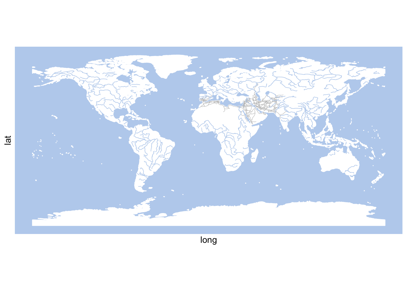

Routes are plotted in grey; rivers — in blue. We will not modify routes in any way with additional data for visualization. Let’s now load network data, which will include the following:

• nodes will be settlements;
• edges will be “routes” that we see on the map, but we will use only values, not the “drawings” of these routes for our analysis. More specifically, our edges data will include connections between places. Here we will need some additional steps.

Let’s load edges first, as they are rather simple (download: althurayya.zip). There is a lot of data that we will not need, so I will filter it out,

edges <- read_delim("./data_temp/althurayya/routes.csv", 
    "\t", escape_double = FALSE, trim_ws = TRUE)

edges <- edges %>%
  mutate(weight = meter) %>%
  select(sToponym, eToponym, weight, meter, terrain, safety)

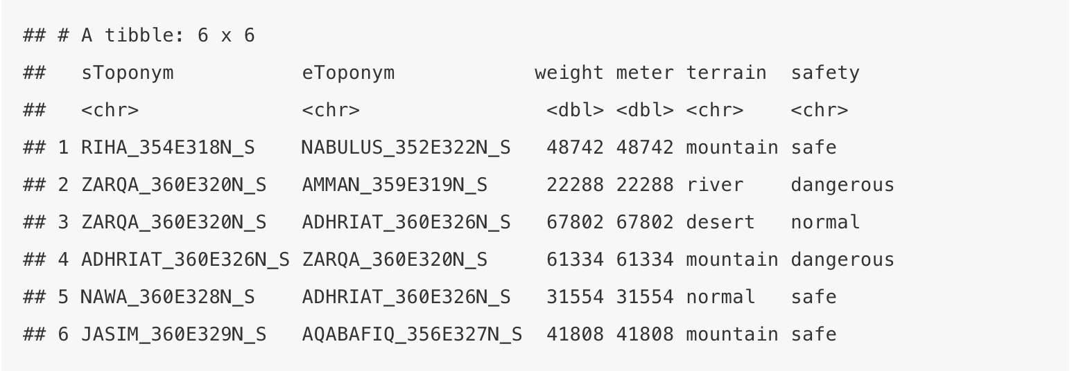
head(edges)

## # A tibble: 6 x 6
##   sToponym           eToponym            weight meter terrain  safety   
##   <chr>              <chr>                <dbl> <dbl> <chr>    <chr>    
## 1 RIHA_354E318N_S    NABULUS_352E322N_S   48742 48742 mountain safe     
## 2 ZARQA_360E320N_S   AMMAN_359E319N_S     22288 22288 river    dangerous
## 3 ZARQA_360E320N_S   ADHRIAT_360E326N_S   67802 67802 desert   normal   
## 4 ADHRIAT_360E326N_S ZARQA_360E320N_S     61334 61334 mountain dangerous
## 5 NAWA_360E328N_S    ADHRIAT_360E326N_S   31554 31554 normal   safe     
## 6 JASIM_360E329N_S   AQABAFIQ_356E327N_S  41808 41808 mountain safe

Here we have sToponym, eToponym, and meter, i.e. the distance from the start-place to the end-place. The “start” and the “end” do not really carry any meaning here as the network is undirected.

We will use the values from meter as weight for now. Below, we will discuss how these values may be modeled in order to make your network more nuanced.

Now, the nodes:

nodes <- read_delim("./data_temp/althurayya/settlements.csv", 
    "\t", escape_double = FALSE, trim_ws = TRUE)

nodes <- nodes %>%
  separate(col=coordinates, into=c("l", "lon", "lat", "r"), sep="([\\[, \\]]+)") %>%
  select(settlement_id, names_eng_translit, region_URI, top_type, lon, lat) %>%
  mutate(lon = as.numeric(lon), lat = as.numeric(lat))

# remove nodes which are not in the network
nwNodes <- unique(c(edges$sToponym, edges$eToponym))

nodes <- nodes %>%
  filter(settlement_id %in% nwNodes)

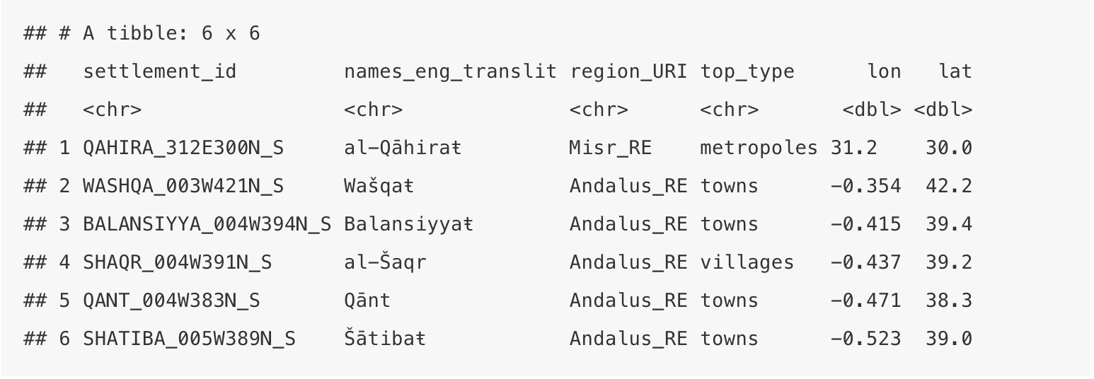
head(nodes)

## # A tibble: 6 x 6
##   settlement_id         names_eng_translit region_URI top_type      lon   lat
##   <chr>                 <chr>              <chr>      <chr>       <dbl> <dbl>
## 1 QAHIRA_312E300N_S     al-Qāhiraŧ         Misr_RE    metropoles 31.2    30.0
## 2 WASHQA_003W421N_S     Wašqaŧ             Andalus_RE towns      -0.354  42.2
## 3 BALANSIYYA_004W394N_S Balansiyyaŧ        Andalus_RE towns      -0.415  39.4
## 4 SHAQR_004W391N_S      al-Šaqr            Andalus_RE villages   -0.437  39.2
## 5 QANT_004W383N_S       Qānt               Andalus_RE towns      -0.471  38.3
## 6 SHATIBA_005W389N_S    Šātibaŧ            Andalus_RE towns      -0.523  39.0

Let’s quickly generate a map with our nodes — so that you have a general idea:

nodesTop <- nodes %>%
  filter(top_type == "metropoles")

annotData <- nodesTop

metropoles <- IslamicWorldBaseBare + 
  geom_point(data = nodes, aes(x=lon, y=lat, col=region_URI), alpha=1, size=0.25) +
  geom_point(data = annotData, aes(x=lon, y=lat), col="red", size=1) +
  geom_label_repel(data = annotData, aes(label = names_eng_translit, x=lon, y=lat)) + 
  coord_sf(xlim=c(min(nodes$lon)-1, max(nodes$lon)+1),
           ylim=c(min(nodes$lat)-1, max(nodes$lat)+1),
                 expand=FALSE)

metropoles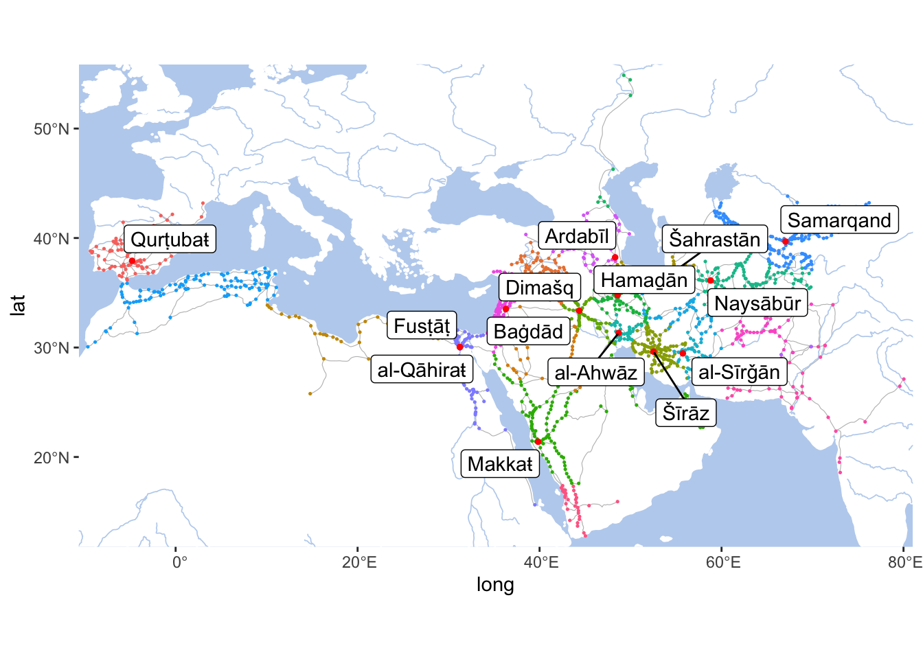

The following lines of code will help you to save your maps without unnecessary information — cut out and keep only the map. There may still be white stripes on the sides, so you may have to need to play around with the width and height parameters.

gt <- ggplot_gtable(ggplot_build(metropoles))
ge <- subset(gt$layout, name == "panel")

ggsave(file=paste0("./files/networks/IW_metropoles.png"),
       # the following line focuses on the graph
       plot=grid.draw(gt[ge$t:ge$b, ge$l:ge$r]),
       # width and height should be experimentally adjusted to remove white space
       dpi=300,width=8.4,height=4.65)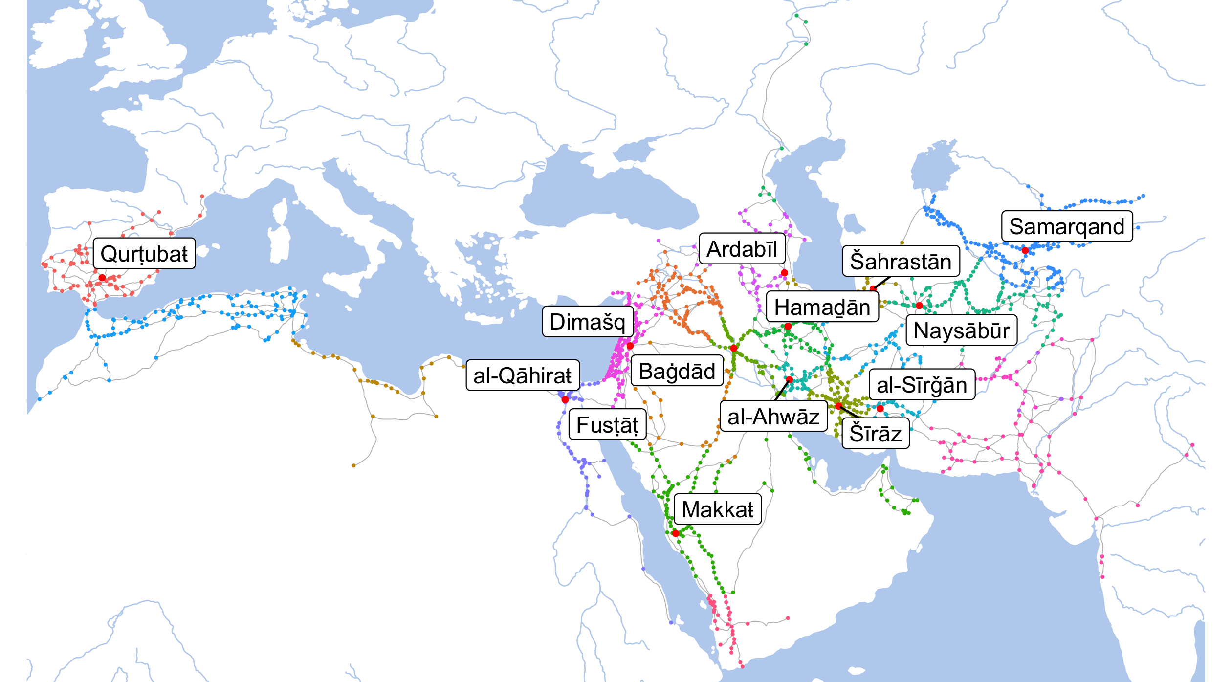

Note: Colors of dots on this map indicate different provinces of the early Islamic world. Considering that borders—in the modern sense—did not exist back then, this is one of the most efficient ways of displaying the extents of regions. White areas effectively indicate uninhabited lands—in most cases, deserts, mountains, or mountainous deserts.

10.4.5 The Network

Now, as we have both the nodes and the edges, we can start our analysis. There are a few things that make sense to begin with:

• look for the most important nodes in the network: i.e. those nodes, through which most other nodes are connected to each other (in practical terms that would mean that most people would travel through those places and, as a result, we may expect that these places would play an important role in cultural exchange); this analysis can be done in a variety of ways—we can use the network as is, or we can apply a variety of modifications that would help us to “encode” some additional historical information that might be missing from the network. By and large, this includes different centrality measures (degree, betweenness, eigenvector centrality, etc.);

• look for most closely interconnected clusters of nodes, which may may help us to understand the historical confines of specific areas, such as provinces, states, conquered territories and the like;

• look for the shortest paths within the network (i.e., how one would travel from one place to another);

• and, if we have relevant data, we can “overplot” other networks on geographical maps (movements of people); in this case, however, the network will be different and we will simply use the map as its layout.

We start by creating a network object in the following manner:

library(igraph)
iwNetwork <- graph_from_data_frame(d=edges, vertices=nodes, directed=FALSE)
iwNetwork

## IGRAPH fa115b7 UNW- 1692 2053 -- 
## + attr: name (v/c), names_eng_translit (v/c), region_URI (v/c),
## | top_type (v/c), lon (v/n), lat (v/n), weight (e/n), meter (e/n),
## | terrain (e/c), safety (e/c)
## + edges from fa115b7 (vertex names):
## [1] NABULUS_352E322N_S --RIHA_354E318N_S         
## [2] AMMAN_359E319N_S   --ZARQA_360E320N_S        
## [3] ZARQA_360E320N_S   --ADHRIAT_360E326N_S      
## [4] ZARQA_360E320N_S   --ADHRIAT_360E326N_S      
## [5] NAWA_360E328N_S    --ADHRIAT_360E326N_S      
## [6] AQABAFIQ_356E327N_S--JASIM_360E329N_S        
## + ... omitted several edges

The description of an igraph object starts with four letters (in our case: UNW-):

• D or U, for a directed or undirected graph
• N for a named graph (where nodes have a name attribute)
• W for a weighted graph (where edges have a weight attribute)
• B for a bipartite (two-mode) graph (where nodes have a type attribute)

In our case, it is UNW-, i.e.: undirected, named, weighted, and not bipartite.

The two numbers that follow (110 444) refer to the number of nodes and edges in the graph. The description also lists node & edge attributes, for example:

• (g/c) - graph-level character attribute
• (v/c) - vertex-level character attribute
• (e/n) - edge-level numeric attribute

igraph objects provide us with an easy access to nodes, edges, and their attributes with the following commands:

head(E(iwNetwork), 20)

## + 20/2053 edges from fa115b7 (vertex names):
##  [1] NABULUS_352E322N_S   --RIHA_354E318N_S         
##  [2] AMMAN_359E319N_S     --ZARQA_360E320N_S        
##  [3] ZARQA_360E320N_S     --ADHRIAT_360E326N_S      
##  [4] ZARQA_360E320N_S     --ADHRIAT_360E326N_S      
##  [5] NAWA_360E328N_S      --ADHRIAT_360E326N_S      
##  [6] AQABAFIQ_356E327N_S  --JASIM_360E329N_S        
##  [7] NAWA_360E328N_S      --JABIYA_360E329N_S       
##  [8] JABIYA_360E329N_S    --JASIM_360E329N_S        
##  [9] ADHRIAT_360E326N_S   --ROUTPOINT0121_362E333N_O
## [10] JASIM_360E329N_S     --ROUTPOINT0121_362E333N_O
## + ... omitted several edges

head(V(iwNetwork), 20)

## + 20/1692 vertices, named, from fa115b7:
##  [1] QAHIRA_312E300N_S      WASHQA_003W421N_S      BALANSIYYA_004W394N_S 
##  [4] SHAQR_004W391N_S       QANT_004W383N_S        SHATIBA_005W389N_S    
##  [7] SARAQUSA_009W416N_S    MURSIYA_011W379N_S     TUTILA_016W420N_S     
## [10] LURQA_017W376N_S       MADINASALIM_024W411N_S BAJJANA_024W369N_S    
## [13] MARIYYA_025W368N_S     WADIHIJARA_031W406N_S  WADIYASH_031W373N_S   
## [16] BAYYASA_034W379N_S     GHARNATA_035W372N_S    LIBIRA_036W372N_S     
## [19] QALARABAH_037W388N_S   JAYYAN_038W377N_S

head(E(iwNetwork)$weight, 20)

##  [1]  48742  22288  67802  61334  31554  41808   5016   6380  81803  42594
## [11]  97452 188149  43254  84816  47117  19536  24577  78493  28113  65632

head(V(iwNetwork)$name, 20)

##  [1] "QAHIRA_312E300N_S"      "WASHQA_003W421N_S"      "BALANSIYYA_004W394N_S" 
##  [4] "SHAQR_004W391N_S"       "QANT_004W383N_S"        "SHATIBA_005W389N_S"    
##  [7] "SARAQUSA_009W416N_S"    "MURSIYA_011W379N_S"     "TUTILA_016W420N_S"     
## [10] "LURQA_017W376N_S"       "MADINASALIM_024W411N_S" "BAJJANA_024W369N_S"    
## [13] "MARIYYA_025W368N_S"     "WADIHIJARA_031W406N_S"  "WADIYASH_031W373N_S"   
## [16] "BAYYASA_034W379N_S"     "GHARNATA_035W372N_S"    "LIBIRA_036W372N_S"     
## [19] "QALARABAH_037W388N_S"   "JAYYAN_038W377N_S"

Keep these commands in mind because they will help you to extract necessary information from graph objects that you create with igraph and reuse them elsewhere.

10.4.6 Measures of centrality

Now we have our network object in the variable called iwNetwork and we can calculate several most common measures of centrality. They should tell us something about the structure of the network and the role of specific nodes. We will return to this in what follows…

10.4.7 The Shortest Path

You may be interested in finding the shortest path within a specific network. We can do that with the same igraph library and put it on the map. Let’s say, we want to find the shortest path from Baghdad (Baġdād) to Damascus (Dimašq). The following code will give us a vector (sequence) of nodes from one point to another. The second line of code extracts IDs of places from a list of values (we will need a simple vector).

baghdad_to_damascus <- shortest_paths(iwNetwork, from = "BAGHDAD_443E333N_S", to = "DIMASHQ_363E335N_S", weights = E(iwNetwork)$weight)$vpath
baghdad_to_damascus <- names(unlist(baghdad_to_damascus))

The shortest path is found with the Dijkstra algorithm, which is currently the most standard way of calculating the shortest path within a network. Essentially, it finds the path between A and B, where the sum of edges (like distance in meters, for example) is the shortest. Therte are plenty of videos on YouTube with the detailed explanations of how it works (for example, this). Please, take a look, understanding how it works may help you to find a way to use it in other contexts.

We can graph this in the following manner (for simplicity, the red line does not follow the actual routes, but draws a straight line between settlements along the path):

path <- tibble(ID = baghdad_to_damascus) %>%
  left_join(nodes, by = c("ID" = "settlement_id"))

annotData <- path

IslamicWorldBaseBare + 
  geom_path(data = annotData, aes(x=lon, y=lat), col="red") + 
  geom_point(data = annotData, aes(x=lon, y=lat), col="red", size=2) +
  geom_label_repel(data = annotData, aes(label = names_eng_translit, x=lon, y=lat)) + 
  coord_sf(xlim=c(min(annotData$lon)-5, max(annotData$lon)+5),
           ylim=c(min(annotData$lat)-3, max(annotData$lat)+3),
                 expand=FALSE)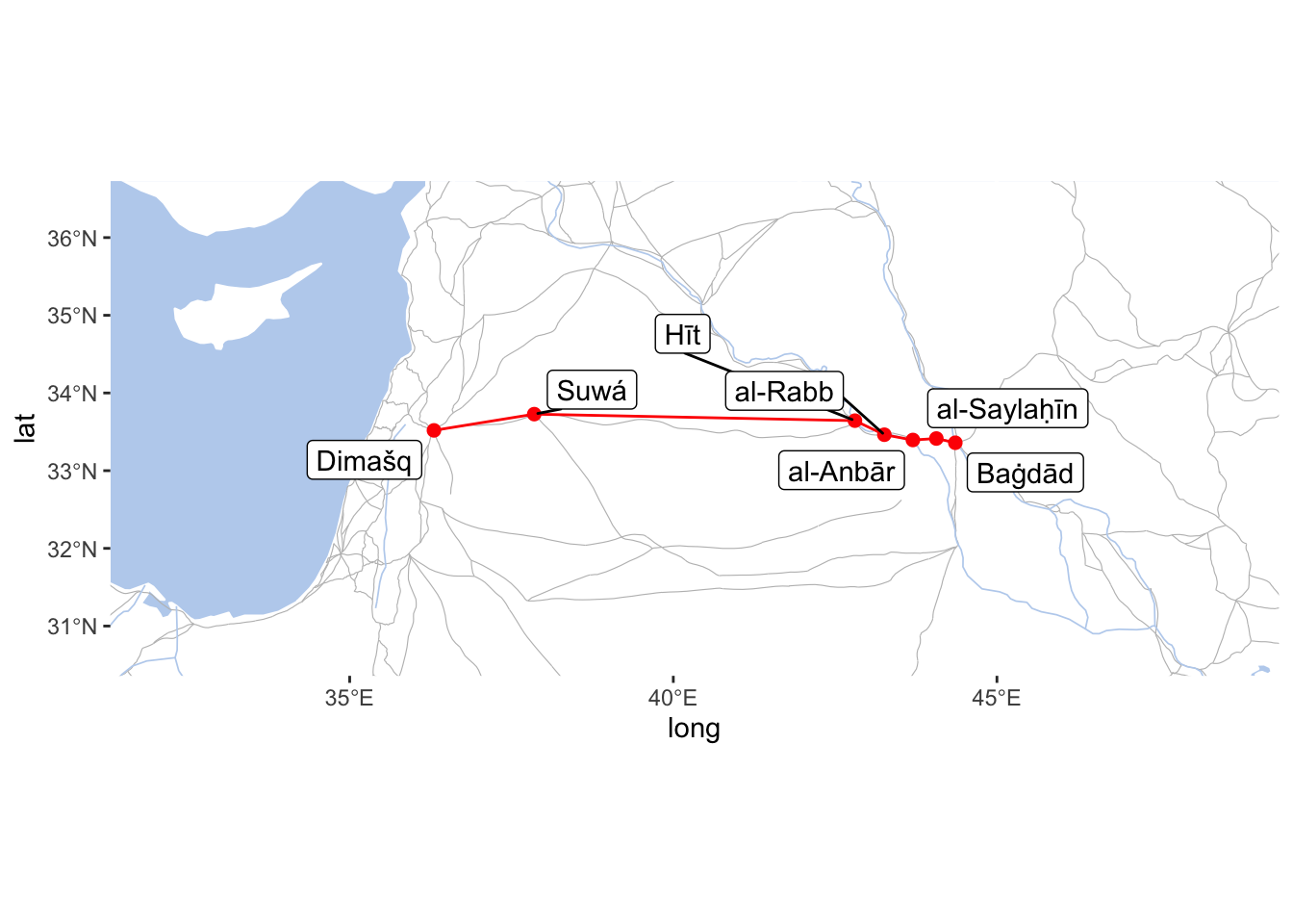

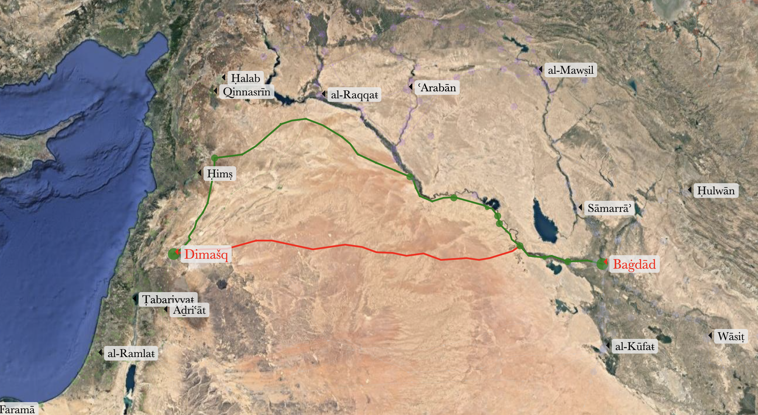
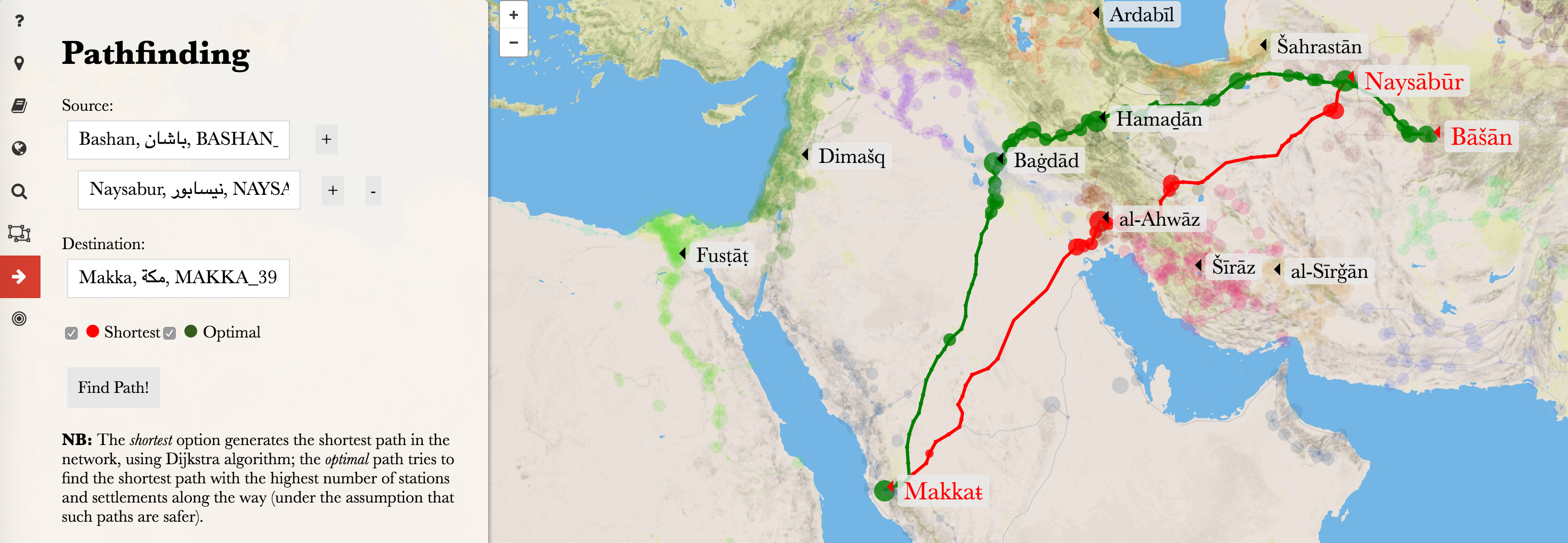
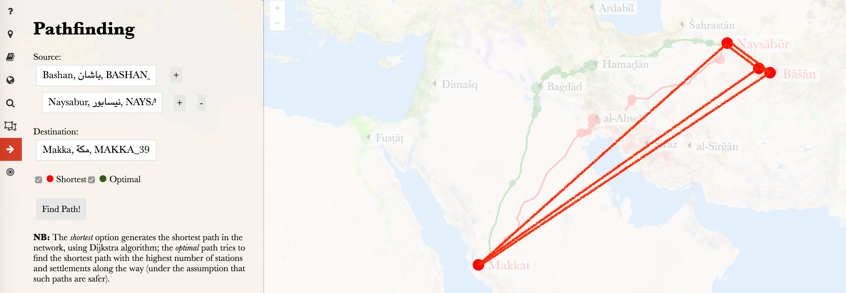
Everything worked as planned, but we need to consider geography and history in order to generate a path that actually makes sense. If we look at the image below, the shortest path (these paths are modeled in althurayya.github.io). The problem with the shortest path is that it is going through the desert, and while it is possible to take this path, this was the path that was avoided as very dangerous. The prefered path was to travel along the Euphrates or the Tigris rivers, and, preferably, along the path with more settlements along the way. On the map below the green path is closer to the prefered option (ideally, it should go through Samarra (Sāmarrāʾ), Mosul (al-Mawṣil), Ar Raqqah (al-Raqqaŧ), and, probably, Aleppo (Ḥalab)).

This is where we can modify some parameters of our network in order to make it work more in line with our geographical and historical knowledge. The Dijkstra algorithm takes into account exclusively the lengths of route sections between the nodes in the network, but we can modify these lengths to make the Dijkstra algorithm work the way we want. This will be the easiest and the most flexible way to re-model our network — we can modify these lengths by introducing additional parameters (multipliers, or dividers). For example, if a node is a “capital” or a “town,” it will be preferable to travel through this node, rather than through a “village” or a “waystation.” Say, we have two equally plausible routes, one between a town and a waystation and another between the same town and another town. We can assign specific multipliers to the types of settlements and use them to adjust the length of paths. Say, a multiplier for “town” will be 0.5, and for a “waystation” — 2. This will make the route between two towns “shorter” that the route between a town and a waystation. As a result, the Dijkstra algorithm will be giving preference to these “shorter” paths. Now, how can we implement this?

These are the types of nodes that we have. We add multipliers that will help us to reduce or to increase “lengths” of routes based on the types of nodes that they connect.

types <- nodes$top_type %>%
  sort() %>% unique()
    
types <- tibble(type = types,
                mltp = c(0.33, 0.25, 1, 1, 0.5, 1, 2, 2, 2))

types

## # A tibble: 9 x 2
##   type         mltp
##   <chr>       <dbl>
## 1 capitals     0.33
## 2 metropoles   0.25
## 3 quarters     1   
## 4 sites        1   
## 5 towns        0.5 
## 6 villages     1   
## 7 waters       2   
## 8 waystations  2   
## 9 xroads       2

First, let’s add these multipliers to our nodes:

nodesM <- nodes %>%
  left_join(types, by = c("top_type" = "type"))

nodesM

## # A tibble: 1,692 x 7
##    settlement_id       names_eng_transl… region_URI top_type     lon   lat  mltp
##    <chr>               <chr>             <chr>      <chr>      <dbl> <dbl> <dbl>
##  1 QAHIRA_312E300N_S   al-Qāhiraŧ        Misr_RE    metropol… 31.2    30.0  0.25
##  2 WASHQA_003W421N_S   Wašqaŧ            Andalus_RE towns     -0.354  42.2  0.5 
##  3 BALANSIYYA_004W394… Balansiyyaŧ       Andalus_RE towns     -0.415  39.4  0.5 
##  4 SHAQR_004W391N_S    al-Šaqr           Andalus_RE villages  -0.437  39.2  1   
##  5 QANT_004W383N_S     Qānt              Andalus_RE towns     -0.471  38.3  0.5 
##  6 SHATIBA_005W389N_S  Šātibaŧ           Andalus_RE towns     -0.523  39.0  0.5 
##  7 SARAQUSA_009W416N_S Saraqūsaŧ         Andalus_RE towns     -0.929  41.6  0.5 
##  8 MURSIYA_011W379N_S  Mursiyaŧ          Andalus_RE towns     -1.11   38.0  0.5 
##  9 TUTILA_016W420N_S   Tuṭīlaŧ           Andalus_RE towns     -1.63   42.0  0.5 
## 10 LURQA_017W376N_S    Lurqaŧ            Andalus_RE towns     -1.73   37.7  0.5 
## # … with 1,682 more rows

We also have additional classification of routes in terms of terrain and safety. We can use these as additional multipliers. (These may be more efficient, but they are more time consuming to create.)

terrainDF <- tibble("terrain" = c("desert", "normal", "mountain", "river"),
                  "mltp"   = c(2, 1, 1.25, 0.75))

terrainDF

## # A tibble: 4 x 2
##   terrain   mltp
##   <chr>    <dbl>
## 1 desert    2   
## 2 normal    1   
## 3 mountain  1.25
## 4 river     0.75

safetyDF <- tibble("safety" = c("dangerous", "safe", "normal"),
                 "mltp"   = c(2, 0.75, 1))

safetyDF

## # A tibble: 3 x 2
##   safety     mltp
##   <chr>     <dbl>
## 1 dangerous  2   
## 2 safe       0.75
## 3 normal     1

Now, we can generate new “weights” for our edges.

Note: there are no strict rules with regard to how you modify your network, your nodes and your edges; it must make sense, so, use your judgement; consult your peers and your advisers; always clearly describe the process of your modifications. For example, the following is happenning below: we multiply the length in meters by the sum of node multipliers (here lower values will turn nodes into magnets of sorts—metropoles and capitals will act as natural attractors); then we multiply the resulting values by the sum of “terrain” and “safety” multipliers (here higher values will make edges “longer”—i.e, routes that go through deserts will become longer than routes ging through a plain).

# simply reloading edges data

edges <- read_delim("./data_temp/althurayya/routes.csv", 
    "\t", escape_double = FALSE, trim_ws = TRUE)

## Parsed with column specification:
## cols(
##   route_id = col_character(),
##   sToponym = col_character(),
##   sToponym_type = col_character(),
##   eToponym = col_character(),
##   eToponym_type = col_character(),
##   terrain = col_character(),
##   safety = col_character(),
##   coordinates = col_character(),
##   meter = col_double()
## )

edges <- edges %>%
  mutate(weight = meter) %>%
  select(sToponym, eToponym, weight, meter, terrain, safety)

head(edges)

## # A tibble: 6 x 6
##   sToponym           eToponym            weight meter terrain  safety   
##   <chr>              <chr>                <dbl> <dbl> <chr>    <chr>    
## 1 RIHA_354E318N_S    NABULUS_352E322N_S   48742 48742 mountain safe     
## 2 ZARQA_360E320N_S   AMMAN_359E319N_S     22288 22288 river    dangerous
## 3 ZARQA_360E320N_S   ADHRIAT_360E326N_S   67802 67802 desert   normal   
## 4 ADHRIAT_360E326N_S ZARQA_360E320N_S     61334 61334 mountain dangerous
## 5 NAWA_360E328N_S    ADHRIAT_360E326N_S   31554 31554 normal   safe     
## 6 JASIM_360E329N_S   AQABAFIQ_356E327N_S  41808 41808 mountain safe

Now, updating the weights based on our multipliers:

nodesL <- nodesM %>%
  select(settlement_id, mltp)

edgesM <- edges %>%
  left_join(nodesL, by = c("sToponym" = "settlement_id")) %>%
  left_join(nodesL, by = c("eToponym" = "settlement_id")) %>%
  left_join(terrainDF, by = c("terrain" = "terrain")) %>%
  left_join(safetyDF, by = c("safety" = "safety")) %>%
  mutate(weight_mod = meter) %>%
  mutate(weight_mod = weight_mod * (mltp.x + mltp.y)) %>%
  mutate(weight_mod = weight_mod * (mltp.x.x + mltp.y.y))

head(edgesM)

## # A tibble: 6 x 11
##   sToponym eToponym weight meter terrain safety mltp.x mltp.y mltp.x.x mltp.y.y
##   <chr>    <chr>     <dbl> <dbl> <chr>   <chr>   <dbl>  <dbl>    <dbl>    <dbl>
## 1 RIHA_35… NABULUS…  48742 48742 mounta… safe     0.5    0.5      1.25     0.75
## 2 ZARQA_3… AMMAN_3…  22288 22288 river   dange…   2      0.5      0.75     2   
## 3 ZARQA_3… ADHRIAT…  67802 67802 desert  normal   2      0.33     2        1   
## 4 ADHRIAT… ZARQA_3…  61334 61334 mounta… dange…   0.33   2        1.25     2   
## 5 NAWA_36… ADHRIAT…  31554 31554 normal  safe     0.5    0.33     1        0.75
## 6 JASIM_3… AQABAFI…  41808 41808 mounta… safe     2      1        1.25     0.75
## # … with 1 more variable: weight_mod <dbl>

Now, let’s try to find the shortest route with our new data:

iwNetworkMod <- graph_from_data_frame(d=edgesM, vertices=nodesM, directed=FALSE)

baghdad_to_damascusMod <- shortest_paths(iwNetworkMod, from = "BAGHDAD_443E333N_S", to = "DIMASHQ_363E335N_S", weights = E(iwNetworkMod)$weight_mod)$vpath
baghdad_to_damascusMod <- names(unlist(baghdad_to_damascusMod))

pathMod <- tibble(ID = baghdad_to_damascusMod) %>%
  left_join(nodes, by = c("ID" = "settlement_id"))

pathModLabels <- pathMod %>%
  mutate(label = names_eng_translit) %>%
  filter(top_type == "metropoles" | top_type == "capitals")

annotData <- pathMod

IslamicWorldBaseBare + 
  geom_path(data = annotData, aes(x=lon, y=lat), col="red") + 
  geom_point(data = annotData, aes(x=lon, y=lat), col="red", size=2) +
  geom_label_repel(data = pathModLabels, aes(label = label, x=lon, y=lat), max.overlaps = 100) + 
  coord_sf(xlim=c(min(annotData$lon)-5, max(annotData$lon)+5),
           ylim=c(min(annotData$lat)-3, max(annotData$lat)+3),
                 expand=FALSE)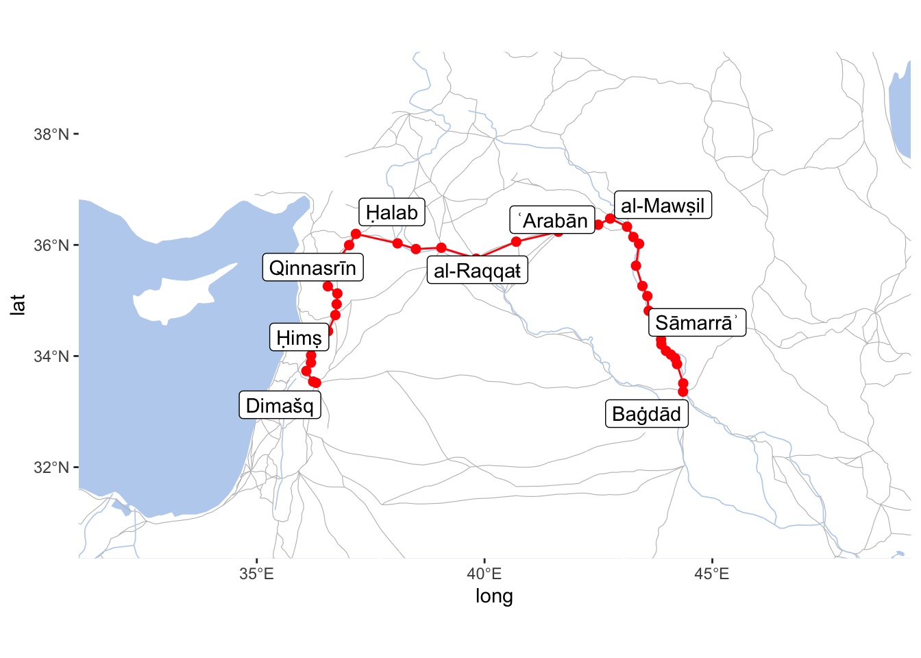

As you can see, the results are quite what we wanted. This is is not the easiest approach to implement, but it will give you full control over modeling different processes within your geographical networks. (Important: the data used in this section is not complete; “terrain” and “safety” classifications are random, except for this specific example.)

10.4.8 Centrality measures, Clusters/Communities

A way to find large components of any network is to apply some cluster analysis algorithms. There are many different algorithms which are included in igraph. One needs to understand how they work and for which purposes they have been developed. For our current context, the following algorithms are most fitting. Please, check additional references at the end of the lesson for more details.

Let’s reload our data. For cluster analysis we will need to modify weights of our edges, since cluster analysis algorithms expect more important edges to have higher weight—in other words, shorter routes must have higher weight than longer ones (for the Dijkstra algorithm we needed the opposite).

I will condense everything in one block:

# file with additional metadata on nodes
mapLayer <- read_delim("./data_temp/althurayya/topMicroUPD.csv", "\t", escape_double = FALSE, trim_ws = TRUE)
mapLayer_Filtered <- mapLayer %>% filter(!is.na(aRegion))
aRegions <- read_delim("./data_temp/althurayya/top_aRegions_VizCenters.csv", "\t", escape_double = FALSE, trim_ws = TRUE)

# processing main data: loading edges and creating a network object
althurayyaE <- read_delim("./data_temp/althurayya/althurayya_edges.csv", "\t", escape_double = FALSE, trim_ws = TRUE) %>%
  mutate(weight = signif(1/length*10000, digits=2))

althurayyaNetwork <- graph_from_data_frame(d=althurayyaE, directed=F)
althurayyaNetwork <- simplify(althurayyaNetwork) # this helps to remove duplicate edges and loop edges

# centrality measures
V(althurayyaNetwork)$degree <- degree(althurayyaNetwork, mode="all")
V(althurayyaNetwork)$centr_eigen <- centr_eigen(althurayyaNetwork, directed=F, normalized=F)$vector
V(althurayyaNetwork)$betweenness <- betweenness(althurayyaNetwork, directed=F)
V(althurayyaNetwork)$centr_betw <- centr_betw(althurayyaNetwork, directed=F, normalized=T)$res

# clustering (selected algorithms) some of these alrgorithms may take a minute of two to run
V(althurayyaNetwork)$cl_walktrap <- as.character(cluster_walktrap(althurayyaNetwork)$membership)
V(althurayyaNetwork)$cl_louvain <- as.character(cluster_louvain(althurayyaNetwork)$membership)

# extract nodes/vertices for mapping
althurayyaNodes <- as_data_frame(althurayyaNetwork, what="vertices")
althurayyaNodes <- althurayyaNodes %>%
  rename(URI = name) %>%
  left_join(mapLayer, by="URI") %>%
  filter(!is.na(aRegion))

head(althurayyaNodes)

##                   URI degree  centr_eigen betweenness centr_betw cl_walktrap
## 1   ABADHA_526E311N_S      2 1.195227e-16      4681.0   8465.361          10
## 2   ABADHA_537E297N_S      2 0.000000e+00      3476.5   9844.930           1
## 3 ABARKATH_673E397N_S      2 0.000000e+00         0.0  42306.633          24
## 4  ABARQUH_532E311N_S      2 0.000000e+00      6596.0   7803.052          84
## 5  ABASKUN_540E370N_S      1 0.000000e+00         0.0      0.000          11
## 6  ABBADAN_482E303N_S      2 2.259505e-09    416626.2 272153.080          19
##   cl_louvain       REG_MESO        aRegion       TR           SEARCH   EN
## 1         25        Fars_RE     SW_Iran_MR   Ābāḏaŧ   Abadha|Arjuman <NA>
## 2         26        Fars_RE     SW_Iran_MR   Ābāḏaŧ           Abadha <NA>
## 3          8 Mawarannahr_RE Mawarannahr_MR  Abārkaṯ Abarkath|Barkath <NA>
## 4         26        Fars_RE     SW_Iran_MR  Abarqūh          Abarquh <NA>
## 5         35      Daylam_RE     NW_Iran_MR  Ābaskūn          Abaskun <NA>
## 6          9        Iraq_RE        Iraq_MR ʿAbbādān          Abbadan <NA>
##       TYPE      LON      LAT     AR       AR_Alt AR_Sort AMBIG TRUETOP   TOPO
## 1    towns 52.66127 31.16430  آباذة آباذة|أرجمان   اباذة     0       0  اباذة
## 2    towns 53.73617 29.78210  آباذة        آباذة   اباذة     0       0  اباذة
## 3 capitals 67.38308 39.79611 أباركث أباركث|بركاث  اباركث     0       1 اباركث
## 4    towns 53.25737 31.15094 أبرقوه       أبرقوه  ابرقوه     0       0 ابرقوه
## 5    towns 54.04327 37.02772 آبسكون       آبسكون  ابسكون     0       0 ابسكون
## 6    towns 48.27394 30.33563 عبادان       عبادان  عبادان     0       0 عبادان

Let’s quickly redo the base layer:

IslamicWorldBase <- ggplot(data=world) +
  geom_sf(fill=colLand, color="black", lwd=0.25) +
  # rivers, aral sea, and routes
  geom_path(data=routes_df, aes(x=long, y=lat, group=id), color=colRout, size=.2) +
  geom_path(data=rivers_df, aes(x=long, y=lat, group=group), color=colWater, alpha=1, size=.3) +
  geom_polygon(data=aral_sea_df, aes(x=long, y=lat, group=group), color=colWater, fill=colWater, size=.2) +
  theme(panel.grid.major=element_line(color=colWater, linetype="dotted", size=0.5),
        panel.background=element_rect(fill=colWater),legend.position="none", panel.border=element_blank())

We now have a lot of new data to check:

# let's filter out the smallest nodes (xroads and waystations)
althurayyaNodesFilt <- althurayyaNodes %>%
    filter(TYPE != "waystations" & TYPE != "sites" & TYPE != "quarters" & TYPE != "waters")

# final map
currentMap <- IslamicWorldBase + 
  geom_encircle(data=mapLayer_Filtered, s_shape=.1, expand=0.01, alpha=.15, aes(x=LON, y=LAT, col=aRegion, fill=aRegion, group=aRegion)) +
  geom_point(data=althurayyaNodesFilt, aes(x=LON, y=LAT, color=cl_louvain), size=0.25, alpha=0.75) +
  annotate("text", label="cl_louvain", x=80, y=12.5, angle=0, hjust=1, vjust=0, size=4, col="black", alpha=1, fontface="bold") +
  coord_sf(xlim=c(min(althurayyaNodesFilt$LON)-1, max(althurayyaNodesFilt$LON)+1),
           ylim=c(min(althurayyaNodesFilt$LAT)-1, max(althurayyaNodesFilt$LAT)+1),
                 expand=FALSE)
  
# and saving
gt <- ggplot_gtable(ggplot_build(currentMap))
ge <- subset(gt$layout, name == "panel")
ggsave(file=paste0("./files/networks/IW_cl_louvain.png"),
       plot=grid.draw(gt[ge$t:ge$b, ge$l:ge$r]),
       dpi=300,width=8.4,height=4.65)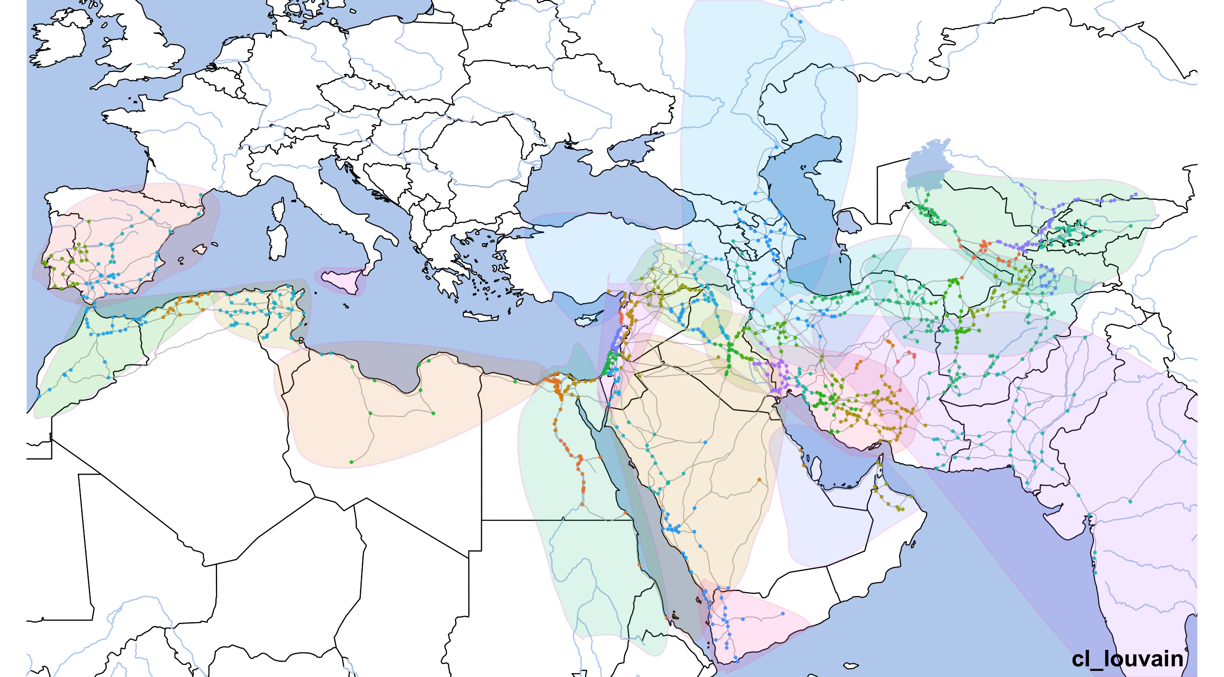

10.4.9 Centrality measures: Degree, Eigenvector, and Betweenness

We have already calculated those (you can find relevant lines of code by searchinf for “degree” and “betweenness”).

Degrees will show us the most highly connected nodes in the network.

althurayyaDegreeLabels <- althurayyaNodes %>%
  slice_max(order_by = degree, n = 15)

minVal = min(althurayyaNodes$degree)
maxVal = max(althurayyaNodes$degree)

lowColor = "darkgreen"
highColor = "red"

# final map
currentMap <- IslamicWorldBase + 
  geom_point(data=althurayyaNodesFilt, aes(x=LON, y=LAT, color=degree, size=degree, alpha=degree)) +
  geom_label_repel(data=althurayyaDegreeLabels, aes(x=LON, y=LAT, label=TR), size=1.5, segment.size=0.25) +
  annotate("text", label="degrees", x=80, y=12.5, angle=0, hjust=1, vjust=0, size=4, col="black", alpha=1, fontface="bold") +
  coord_sf(xlim=c(min(althurayyaNodesFilt$LON)-1, max(althurayyaNodesFilt$LON)+1),
           ylim=c(min(althurayyaNodesFilt$LAT)-1, max(althurayyaNodesFilt$LAT)+1),
                 expand=FALSE) +
  scale_colour_gradient(low=lowColor, high=highColor) +
  scale_size_continuous(range=c(0.001,3), limits=c(minVal,maxVal))

  
# and saving
gt <- ggplot_gtable(ggplot_build(currentMap))
ge <- subset(gt$layout, name == "panel")
ggsave(file=paste0("./files/networks/IW_degrees.png"),
       plot=grid.draw(gt[ge$t:ge$b, ge$l:ge$r]),
       dpi=300,width=8,height=4.6)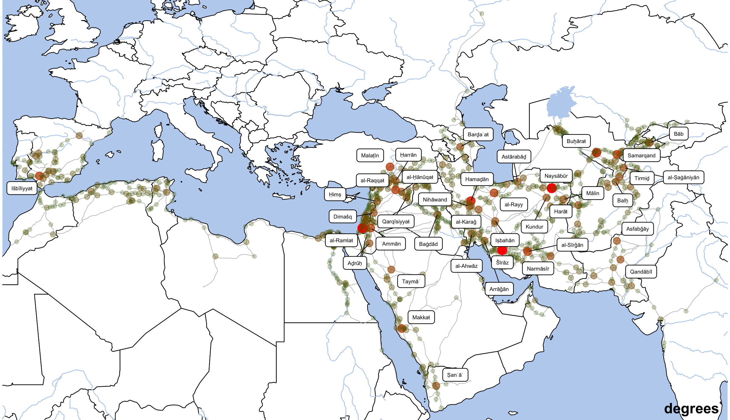

Eienvector centrality

althurayyaDegreeLabels <- althurayyaNodes %>%
  slice_max(order_by = centr_betw, n = 10)

minVal = min(althurayyaNodes$centr_betw)
maxVal = max(althurayyaNodes$centr_betw)

lowColor = "darkgreen"
highColor = "red"

# final map
currentMap <- IslamicWorldBase + 
  geom_point(data=althurayyaNodes, aes(x=LON, y=LAT, color=centr_betw, size=centr_betw, alpha=centr_betw)) +
  geom_label_repel(data=althurayyaDegreeLabels, aes(x=LON, y=LAT, label=TR), size=1.5, segment.size=0.25, max.overlaps = 100) +
  annotate("text", label="centr betweenness", x=80, y=12.5, angle=0, hjust=1, vjust=0, size=4, col="black", alpha=1, fontface="bold") +
  coord_sf(xlim=c(min(althurayyaNodesFilt$LON)-1, max(althurayyaNodesFilt$LON)+1),
           ylim=c(min(althurayyaNodesFilt$LAT)-1, max(althurayyaNodesFilt$LAT)+1),
                 expand=FALSE) +
  scale_colour_gradient(low=lowColor, high=highColor) +
  scale_size_continuous(range=c(0.001,3), limits=c(minVal,maxVal))

# and saving
gt <- ggplot_gtable(ggplot_build(currentMap))
ge <- subset(gt$layout, name == "panel")
ggsave(file=paste0("./files/networks/IW_centr_betw.png"),
       plot=grid.draw(gt[ge$t:ge$b, ge$l:ge$r]),
       dpi=300,width=8,height=4.6)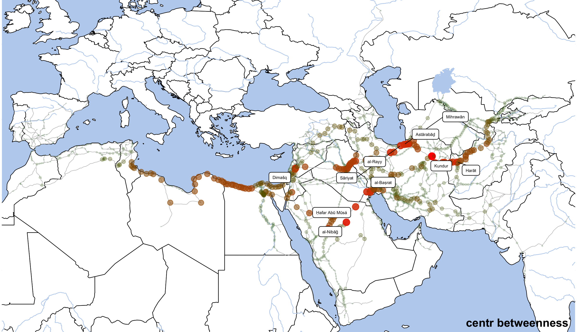

althurayyaDegreeLabels <- althurayyaNodes %>%
  slice_max(order_by = centr_eigen, n = 5)

minVal = min(althurayyaNodes$centr_eigen)
maxVal = max(althurayyaNodes$centr_eigen)

lowColor = "darkgreen"
highColor = "red"

# final map
currentMap <- IslamicWorldBase + 
  geom_point(data=althurayyaNodesFilt, aes(x=LON, y=LAT, color=centr_eigen, size=centr_eigen, alpha=centr_eigen)) +
  geom_label_repel(data=althurayyaDegreeLabels, aes(x=LON, y=LAT, label=TR), size=1.5, segment.size=0.25, max.overlaps = 100) +
  annotate("text", label="centr eigenvector", x=80, y=12.5, angle=0, hjust=1, vjust=0, size=4, col="black", alpha=1, fontface="bold") +
  coord_sf(xlim=c(min(althurayyaNodesFilt$LON)-1, max(althurayyaNodesFilt$LON)+1),
           ylim=c(min(althurayyaNodesFilt$LAT)-1, max(althurayyaNodesFilt$LAT)+1),
                 expand=FALSE) +
  scale_colour_gradient(low=lowColor, high=highColor) +
  scale_size_continuous(range=c(0.001,3), limits=c(minVal,maxVal))

  
# and saving
gt <- ggplot_gtable(ggplot_build(currentMap))
ge <- subset(gt$layout, name == "panel")
ggsave(file=paste0("./files/networks/IW_centr_eigen.png"),
       plot=grid.draw(gt[ge$t:ge$b, ge$l:ge$r]),
       dpi=300,width=8,height=4.6)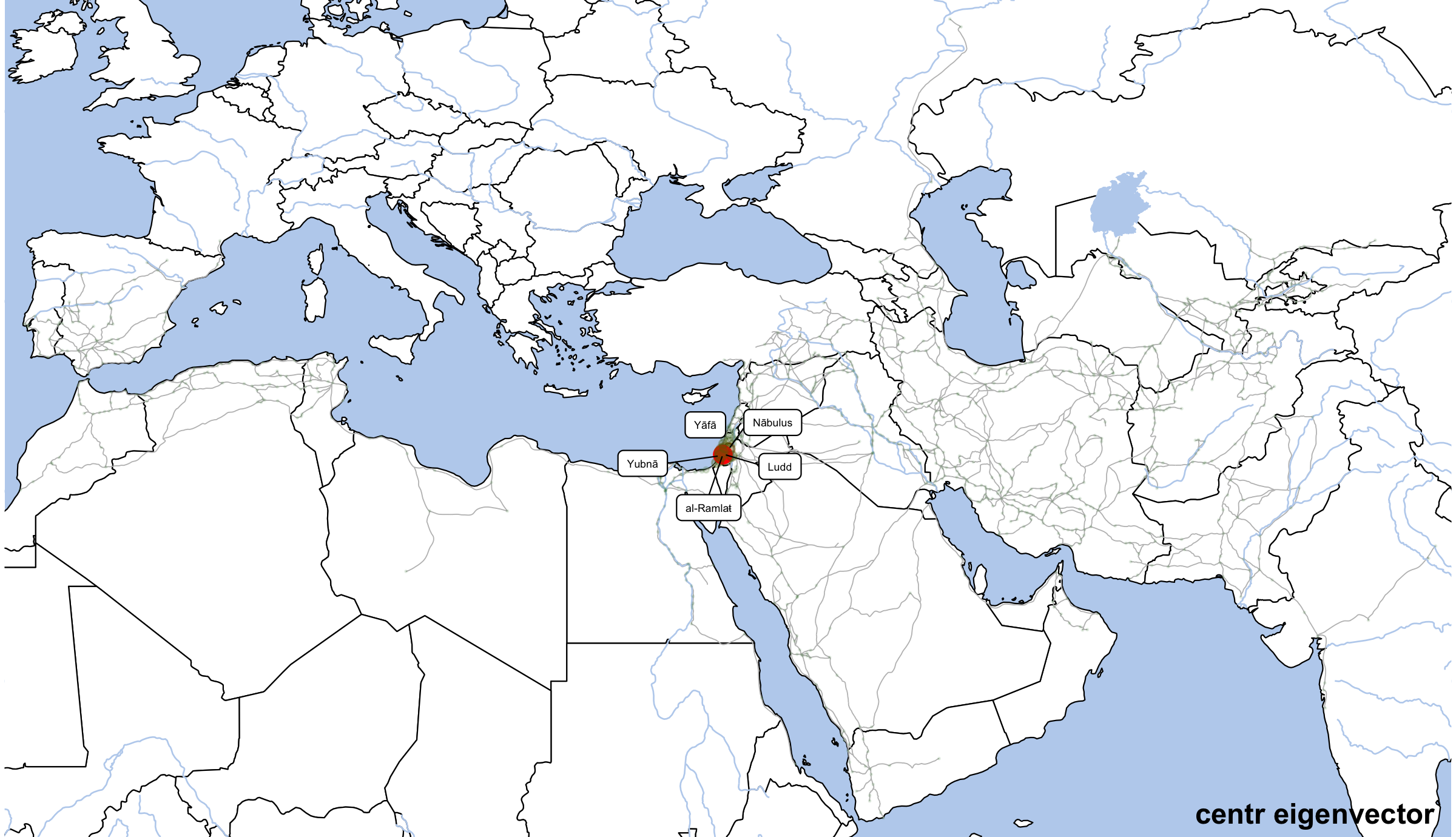

This is a very large network. We can try to reduce it—take a closer look at a specific region.

 [1] "Fars_RE"        "Sind_RE"        "Mawarannahr_RE" "Iraq_RE"        "Daylam_RE"      "Misr_RE"        "Khuzistan_RE"   "Jibal_RE"       "Khurasan_RE"   
[10] "Rihab_RE"       "Andalus_RE"     "Mafaza_RE"      "JaziratArab_RE" "BadiyatArab_RE" "Yaman_RE"       "Sham_RE"        "Aqur_RE"        "Maghrib_RE"    
[19] "Barqa_RE"       "Kirman_RE"      "Khazar_RE"      "Sijistan_RE"    "Rum_RE"         "Ifriqiyya_RE"   "Farghana"       "Iraq"           "Misr" 

northEast <- mapLayer_Filtered %>%
  filter(grepl("Mawarannahr_RE|Khurasan_RE", REG_MESO))

althurayyaE_northEast <- althurayyaE %>%
  filter(source %in% northEast$URI & target %in% northEast$URI)

althurayyaNetwork <- graph_from_data_frame(d=althurayyaE_northEast, directed=F)

# centrality measures
V(althurayyaNetwork)$degree <- degree(althurayyaNetwork, mode="all")
V(althurayyaNetwork)$centr_degree <- centr_degree(althurayyaNetwork, mode="all", normalized=T)$res
V(althurayyaNetwork)$centr_eigen <- centr_eigen(althurayyaNetwork, directed=F, normalized=F)$vector
V(althurayyaNetwork)$betweenness <- betweenness(althurayyaNetwork, directed=F)
V(althurayyaNetwork)$centr_betw <- centr_betw(althurayyaNetwork, directed=F, normalized=T)$res

# clustering (selected algorithms) some of these alrgorithms may take a minute of two to run
V(althurayyaNetwork)$cl_walktrap <- as.character(cluster_walktrap(althurayyaNetwork)$membership)
V(althurayyaNetwork)$cl_louvain <- as.character(cluster_louvain(althurayyaNetwork)$membership)

# extract nodes/vertices for mapping
althurayyaNodes <- as_data_frame(althurayyaNetwork, what="vertices")
althurayyaNodes <- althurayyaNodes %>%
  rename(URI = name) %>%
  left_join(mapLayer, by="URI") %>%
  filter(!is.na(aRegion))

# DEGREE

althurayyaDegreeLabels <- althurayyaNodes %>%
  slice_max(order_by = degree, n = 15)

minVal = min(althurayyaNodes$degree)
maxVal = max(althurayyaNodes$degree)

lowColor = "darkgreen"
highColor = "red"

# final map
currentMap <- IslamicWorldBase + 
  geom_point(data=althurayyaNodes, aes(x=LON, y=LAT, color=degree, size=degree, alpha=degree)) +
  geom_label_repel(data=althurayyaDegreeLabels, aes(x=LON, y=LAT, label=TR), size=1.5, segment.size=0.25) +
  annotate("text", label="degrees", x=80, y=12.5, angle=0, hjust=1, vjust=0, size=4, col="black", alpha=1, fontface="bold") +
  coord_sf(xlim=c(min(althurayyaNodes$LON)-1, max(althurayyaNodes$LON)+1),
           ylim=c(min(althurayyaNodes$LAT)-1, max(althurayyaNodes$LAT)+1),
                 expand=FALSE) +
  scale_colour_gradient(low=lowColor, high=highColor) +
  scale_size_continuous(range=c(0.001,3), limits=c(minVal,maxVal))

# and saving
gt <- ggplot_gtable(ggplot_build(currentMap))
ge <- subset(gt$layout, name == "panel")
ggsave(file=paste0("./files/networks/IW_NorthEast_Degree.png"),
       plot=grid.draw(gt[ge$t:ge$b, ge$l:ge$r]),
       dpi=300,width=8,height=4.6)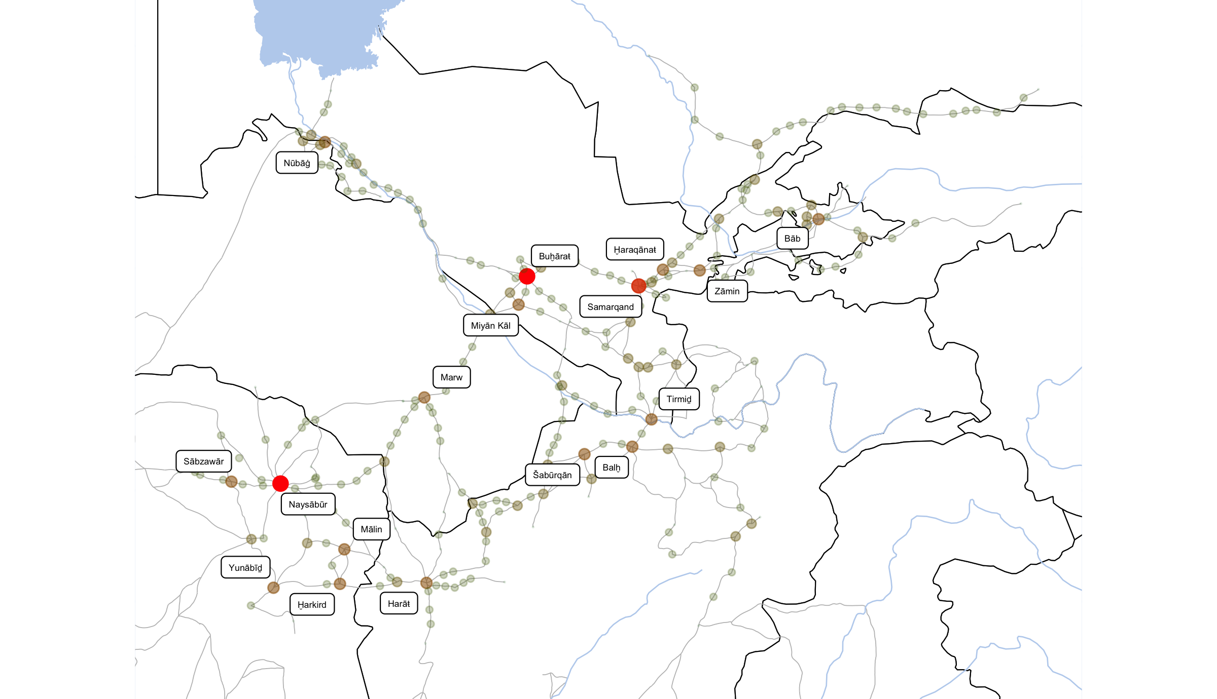

# EIGENVECTOR

althurayyaDegreeLabels <- althurayyaNodes %>%
  slice_max(order_by = centr_eigen, n = 15)

minVal = min(althurayyaNodes$centr_eigen)
maxVal = max(althurayyaNodes$centr_eigen)

lowColor = "darkgreen"
highColor = "red"

# final map
currentMap <- IslamicWorldBase + 
  geom_point(data=althurayyaNodes, aes(x=LON, y=LAT, color=centr_eigen, size=centr_eigen, alpha=centr_eigen)) +
  geom_label_repel(data=althurayyaDegreeLabels, aes(x=LON, y=LAT, label=TR), size=1.5, segment.size=0.25, max.overlaps = 100) +
  annotate("text", label="degrees", x=80, y=12.5, angle=0, hjust=1, vjust=0, size=4, col="black", alpha=1, fontface="bold") +
  coord_sf(xlim=c(min(althurayyaNodes$LON)-1, max(althurayyaNodes$LON)+1),
           ylim=c(min(althurayyaNodes$LAT)-1, max(althurayyaNodes$LAT)+1),
                 expand=FALSE) +
  scale_colour_gradient(low=lowColor, high=highColor) +
  scale_size_continuous(range=c(0.001,3), limits=c(minVal,maxVal))

# and saving
gt <- ggplot_gtable(ggplot_build(currentMap))
ge <- subset(gt$layout, name == "panel")
ggsave(file=paste0("./files/networks/IW_NorthEast_centr_eigen.png"),
       plot=grid.draw(gt[ge$t:ge$b, ge$l:ge$r]),
       dpi=300,width=8,height=4.6)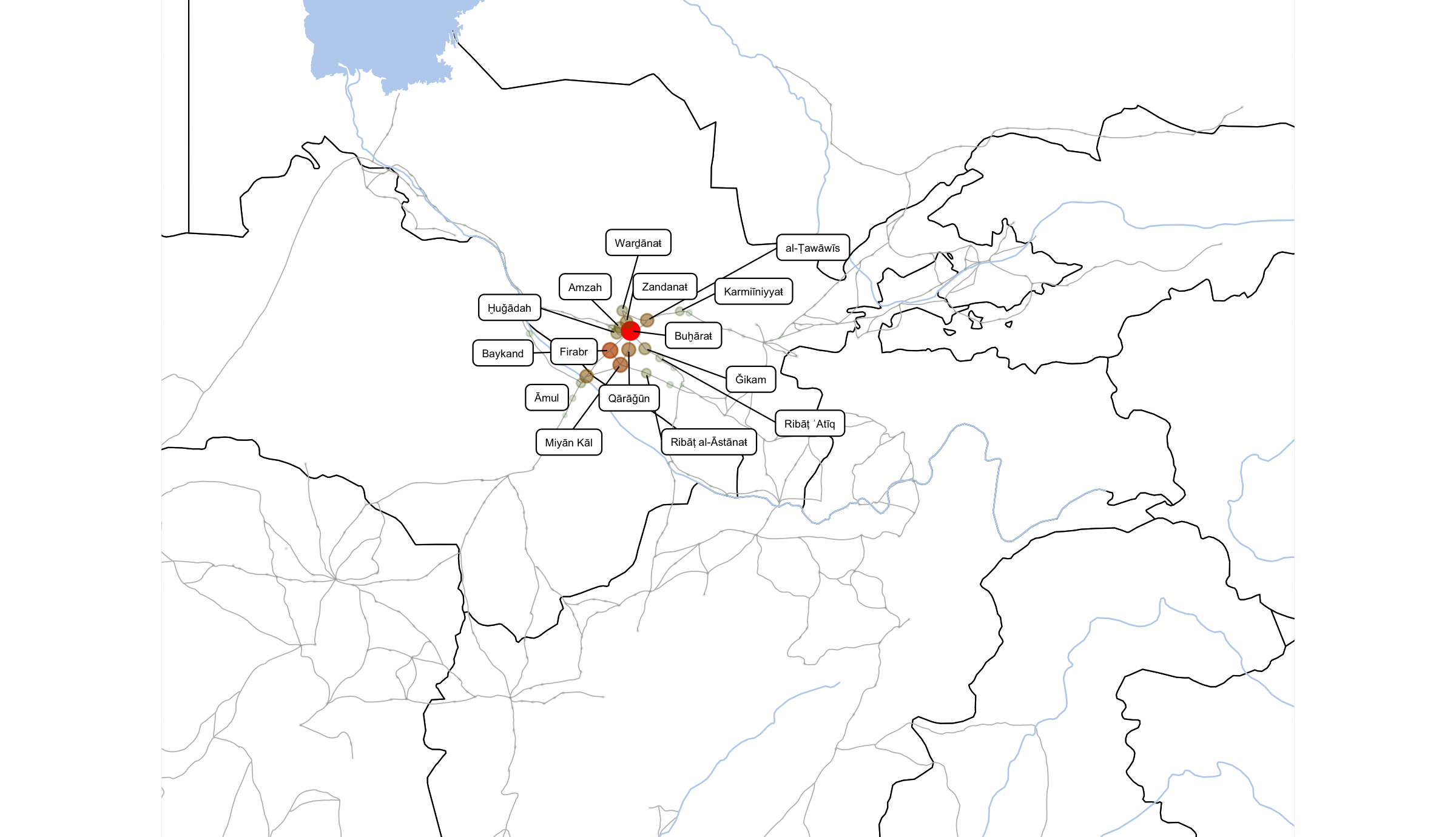

# BETWEENNESS

althurayyaDegreeLabels <- althurayyaNodes %>%
  slice_max(order_by = centr_betw, n = 15)

minVal = min(althurayyaNodes$centr_betw)
maxVal = max(althurayyaNodes$centr_betw)

lowColor = "darkgreen"
highColor = "red"

# final map
currentMap <- IslamicWorldBase + 
  geom_point(data=althurayyaNodes, aes(x=LON, y=LAT, color=centr_betw, size=centr_betw, alpha=centr_betw)) +
  geom_label_repel(data=althurayyaDegreeLabels, aes(x=LON, y=LAT, label=TR), size=1.5, segment.size=0.25, max.overlaps = 100) +
  annotate("text", label="degrees", x=80, y=12.5, angle=0, hjust=1, vjust=0, size=4, col="black", alpha=1, fontface="bold") +
  coord_sf(xlim=c(min(althurayyaNodes$LON)-1, max(althurayyaNodes$LON)+1),
           ylim=c(min(althurayyaNodes$LAT)-1, max(althurayyaNodes$LAT)+1),
                 expand=FALSE) +
  scale_colour_gradient(low=lowColor, high=highColor) +
  scale_size_continuous(range=c(0.001,3), limits=c(minVal,maxVal))

# and saving
gt <- ggplot_gtable(ggplot_build(currentMap))
ge <- subset(gt$layout, name == "panel")
ggsave(file=paste0("./files/networks/IW_NorthEast_centr_betws.png"),
       plot=grid.draw(gt[ge$t:ge$b, ge$l:ge$r]),
       dpi=300,width=8,height=4.6)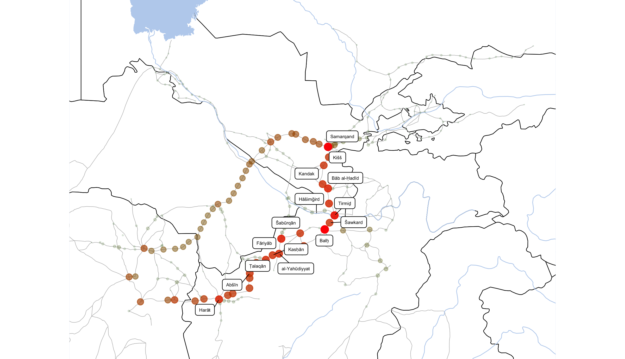

10.4.10 Sparsifying a Network

In some cases your network may be too dense. This will effecively mean that you will not be able to get anything useful from social network analysis methods. What one needs to do in this case is to make the network more sparse. There is a number of ways how one can do this. Ideally, one needs to remodel the network by revising parameters that go into the weights of edges. The simplest way to “sparsify” a network is by deleting edges whose weight is below a certain threshold. In the example below, edges whose value is below mean are deleted from the network. As a result the network should break down into more distinct communities (or, actually, disconnected components).

cut.off <- mean(E(iwNetwork)$weight)

summary(E(iwNetwork)$weight)

##    Min. 1st Qu.  Median    Mean 3rd Qu.    Max. 
##    1687   23842   38387   55530   62771  861693

cutt.off <- 62771
iwNetwork_sparse <- delete_edges(iwNetwork, E(iwNetwork)[weight > cut.off])

Let’s try to map these disconnected components:

cut.off <- 62771 # 1687   23842   38387   55530   62771  861693 
fileName <- paste0("./files/networks/IW_sparse_75f.png")
iwNetwork_sparse <- delete_edges(iwNetwork, E(iwNetwork)[weight >= cut.off])

nodesLight <- nodes %>%
  select(settlement_id, lon, lat, top_type)

edges_sparce <- as_data_frame(iwNetwork_sparse, what="edges") %>%
  select(from, to) %>%
  left_join(nodesLight, by = c("from" = "settlement_id")) %>%
  left_join(nodesLight, by = c("to" = "settlement_id")) %>%
  filter(top_type.x != "waystations" & top_type.x != "xroads") %>%
  filter(top_type.y != "waystations" & top_type.y != "xroads")
  
currentMap <- IslamicWorldBase + 
  geom_segment(data = edges_sparce, aes(x=lon.x, y=lat.x, xend=lon.y, yend=lat.y), col="red", size=0.5) +
  coord_sf(xlim=c(min(nodes$lon)-1, max(nodes$lon)+1),
           ylim=c(min(nodes$lat)-1, max(nodes$lat)+1),
                 expand=FALSE)

gt <- ggplot_gtable(ggplot_build(currentMap))
ge <- subset(gt$layout, name == "panel")

ggsave(file=fileName,
       # the following line focuses on the graph
       plot=grid.draw(gt[ge$t:ge$b, ge$l:ge$r]),
       # width and height should be experimentally adjusted to remove white space
       dpi=300,width=8.4,height=4.65)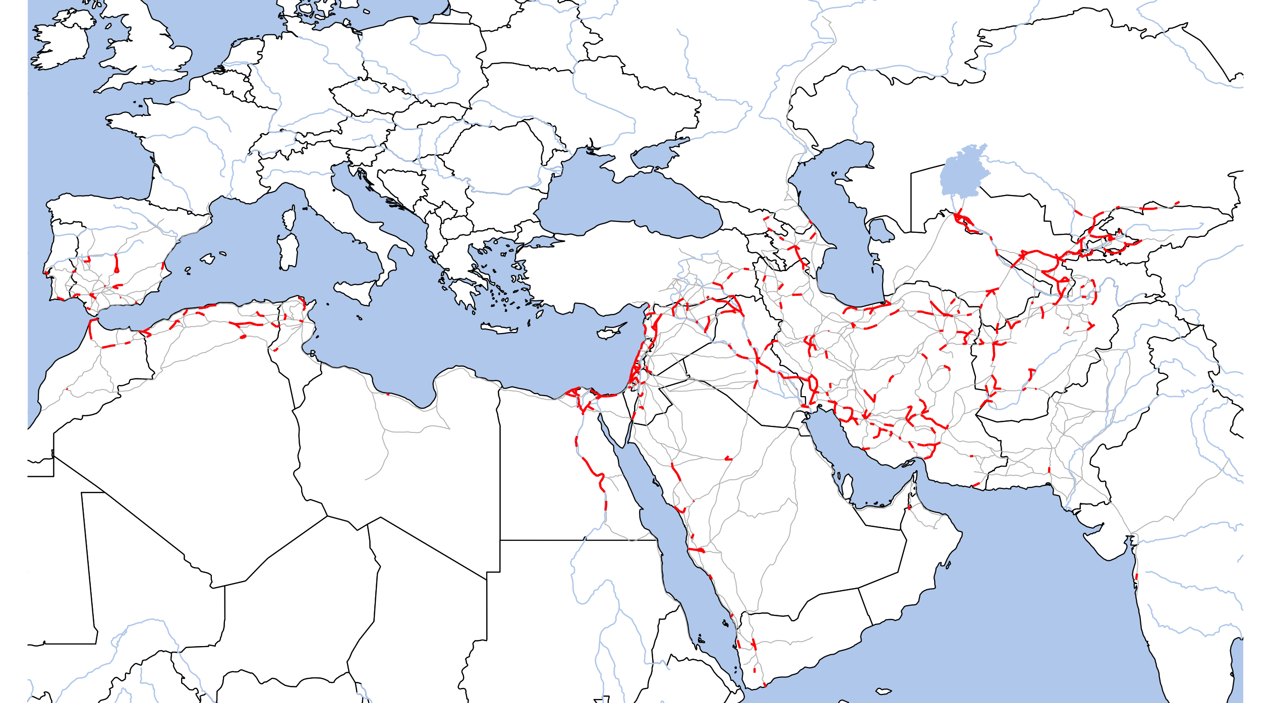

10.4.11 Other networks on maps

Another valuable—perhaps even most valuable—combination of SNA and GIS is mapping other kinds of data as geographical networks. Let’s take a look at the following example:

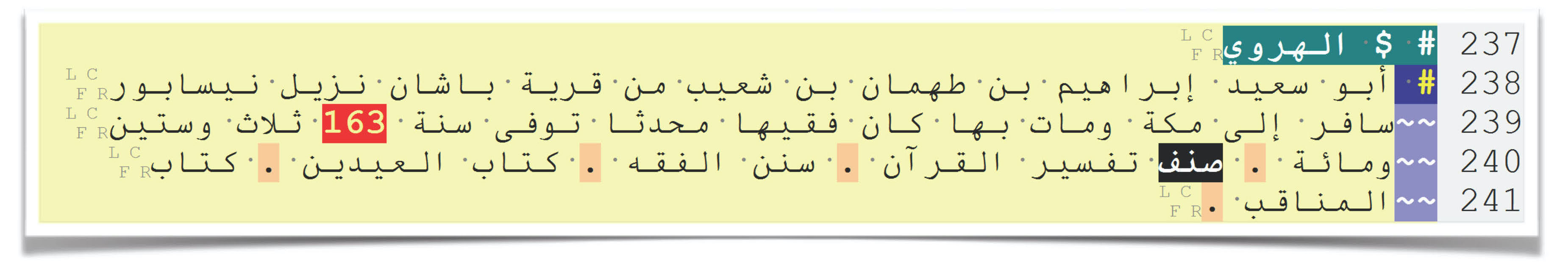
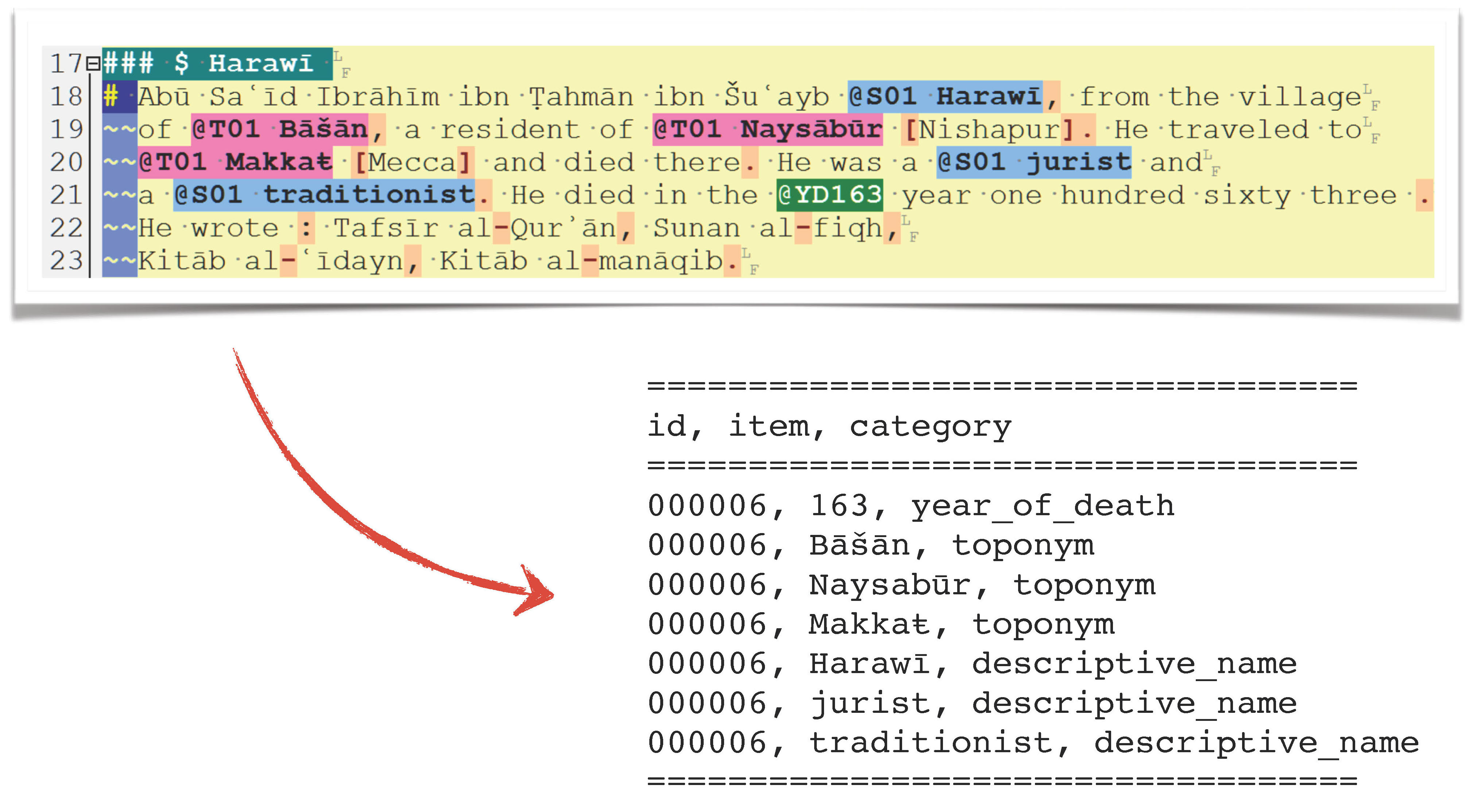
Let’s create networks from the data.

TI_GeoData <- read_delim("./data_temp/althurayya/TI_GeoData_for_R.csv", "\t", escape_double = FALSE, trim_ws = TRUE)
head(TI_GeoData)

## # A tibble: 6 x 3
##   BIO      ITEM   TYPE    
##   <chr>    <chr>  <chr>   
## 1 TI000047 50     DEATH_AH
## 2 TI000048 50     DEATH_AH
## 3 TI000048 البصرة TOPO_PR 
## 4 TI000049 50     DEATH_AH
## 5 TI000050 50     DEATH_AH
## 6 TI000051 50     DEATH_AH

The structure of this data file is as follows: BIO — id of a biography (i.e., a person); ITEM includes a value of a data type defined in the column TYPE. TYPE includes the following values: 1) DEATH_AH—decade of the death of a biographee, according to the Islamic hijrī calendar (anno hegirae); TOPO_PR—a place with which a person is closely associated (“resident of …”); TOPO_SE—a place with which a person is associated (“visitor of …”).

We can split our data into two data frames: with dates and with toponyms.

# split > ID_Dates and ID_TOPO
TIdates <- TI_GeoData %>%
  filter(TYPE=="DEATH_AH") %>%
  rename(DEATH = ITEM)
  
TIdates$DEATH <- as.numeric(TIdates$DEATH)

TIgeoData <- TI_GeoData %>%
  filter(TYPE=="TOPO_PR" | TYPE=="TOPO_SE") %>%
  rename(TOPO = ITEM)

Let’s generate a network on the level of primary toponyms (not regional):

NW_Data_Settl <- data.frame()
idVector = unique(TIgeoData$BIO)

TIgeoDataRichTOP <- TIgeoData %>%
  left_join(mapLayer, by="TOPO") %>%
  filter(!is.na(aRegion)) %>%
  select(BIO, URI) %>%
  unique()

# the following loop is quite slow; use it as a reference for similar cases
# for (ID in idVector){
#   temp <- TIgeoDataRichTOP %>%
#     filter(BIO==ID)
# 
#   if(nrow(temp) > 1){
# 
#     rows <- t(combn(sort(unique(temp$URI)), 2)) %>%
#       as.data.frame() %>%
#       mutate(BIO=ID) %>%
#       rename(FROM=V1) %>%
#       rename(TO=V2) %>%
#       select(BIO, FROM, TO)
# 
#     NW_Data_Settl <- rbind(NW_Data_Settl, rows)
#   }
# }

#saveRDS(NW_Data_Settl, "./data_temp/althurayya/TI_generated_edges.rds")

NW_Data_Settl <- readRDS("./data_temp/althurayya/TI_generated_edges.rds")
head(NW_Data_Settl)

##        BIO             FROM               TO
## 1 TI000052 BASRA_477E304N_S HIJAZ_390E235N_R
## 2 TI000052 BASRA_477E304N_S         Yaman_RE
## 3 TI000052 HIJAZ_390E235N_R         Yaman_RE
## 4 TI000053           Rum_RE          Sham_RE
## 5 TI000054     Ifriqiyya_RE       Maghrib_RE
## 6 TI000054     Ifriqiyya_RE          Misr_RE

The most important line of code in the chunk above is t(combn(sort(unique(temp$URI)), 2)) — it allows you to generate all possible pairs from a list/vector of values. Let’s take a closer look at a smaller example:

vectorWithNodes <- c("Baghdad", "Nishapur", "Basra", "Damascus", "Cairo")
  
edgesGenerated <- t(combn(sort(unique(vectorWithNodes)), 2)) %>%
  as.data.frame() %>%
  rename(FROM=V1) %>%
  rename(TO=V2) %>%
  select(FROM, TO)

edgesGenerated

##        FROM       TO
## 1   Baghdad    Basra
## 2   Baghdad    Cairo
## 3   Baghdad Damascus
## 4   Baghdad Nishapur
## 5     Basra    Cairo
## 6     Basra Damascus
## 7     Basra Nishapur
## 8     Cairo Damascus
## 9     Cairo Nishapur
## 10 Damascus Nishapur

Now, let’s go back to our data and create a network from it: 1) we need to calculate weights of edges, by counting the number of the same edges; 2) create a network object and run the same analyses that we did before; 3) then we can map it.

NW_Data_Final <- NW_Data_Settl %>%
  group_by(FROM, TO) %>%
  summarize(WEIGHT = n())

head(NW_Data_Final)

## # A tibble: 6 x 3
## # Groups:   FROM [1]
##   FROM               TO                  WEIGHT
##   <chr>              <chr>                <int>
## 1 ABARQUH_532E311N_S BAGHDAD_443E333N_S       5
## 2 ABARQUH_532E311N_S BASRA_477E304N_S         1
## 3 ABARQUH_532E311N_S DIMASHQ_363E335N_S       3
## 4 ABARQUH_532E311N_S FASA_536E289N_S          1
## 5 ABARQUH_532E311N_S HAMADHAN_485E347N_S      2
## 6 ABARQUH_532E311N_S HARRAN_390E368N_S        3

Now, the network and the analyses:

NW_Final <- graph_from_data_frame(d=NW_Data_Final, directed=F)

# centrality measures
V(NW_Final)$degree <- degree(NW_Final, mode="all")

# clustering (selected algorithms) some of these alrgorithms may take a minute of two to run
V(NW_Final)$cl_walktrap <- as.character(cluster_walktrap(NW_Final)$membership)
V(NW_Final)$cl_leading_eigen <- as.character(cluster_leading_eigen(NW_Final)$membership)
#V(NW_Final)$cl_edge_betweenness <- as.character(cluster_edge_betweenness(NW_Final)$membership) # too slow
V(NW_Final)$cl_fast_greedy <- as.character(cluster_fast_greedy(NW_Final)$membership) # too slow
V(NW_Final)$cl_louvain <- as.character(cluster_louvain(NW_Final)$membership)

# extract nodes/vertices for mapping
NW_Final_Nodes <- as_data_frame(NW_Final, what="vertices")
NW_Final_Nodes <- NW_Final_Nodes %>%
  rename(URI = name) %>%
  left_join(mapLayer, by="URI")

head(NW_Final_Nodes)

##                      URI degree cl_walktrap cl_leading_eigen cl_fast_greedy
## 1     ABARQUH_532E311N_S     27           1                1              2
## 2     ABBADAN_482E303N_S     33           1                3              2
## 3       ABHAR_492E361N_S     19           1                3              3
## 4     ABIWARD_595E372N_S     29           1                1              2
## 5      ADHANA_353E369N_S     43           1                3              2
## 6 ADHARBAYJAN_479E382N_R    136           3                1              2
##   cl_louvain    REG_MESO    aRegion         TR      SEARCH   EN        TYPE
## 1          2     Fars_RE SW_Iran_MR    Abarqūh     Abarquh <NA>       towns
## 2          2     Iraq_RE    Iraq_MR   ʿAbbādān     Abbadan <NA>       towns
## 3          3    Jibal_RE NW_Iran_MR      Abhar       Abhar <NA>       towns
## 4          2 Khurasan_RE NE_Iran_MR    Abīward     Abiward <NA>       towns
## 5          2     Sham_RE    Sham_MR     Aḏanaŧ      Adhana <NA> waystations
## 6          4    Rihab_RE    Qabq_MR Aḏarbayǧān Adharbayjan <NA>     regions
##        LON      LAT       AR   AR_Alt  AR_Sort AMBIG TRUETOP     TOPO
## 1 53.25737 31.15094   أبرقوه   أبرقوه   ابرقوه     0       0   ابرقوه
## 2 48.27394 30.33563   عبادان   عبادان   عبادان     0       0   عبادان
## 3 49.23473 36.15722     أبهر     أبهر     ابهر     0       0     ابهر
## 4 59.59733 37.27000   أبيورد   أبيورد   ابيورد     0       0   ابيورد
## 5 35.34272 36.96023     أذنة     أذنة     اذنة     0       0     اذنة
## 6 47.95801 38.24076 أذربيجان أذربيجان اذربيجان     0       1 اذربيجان

Now, we can map results of our analysis:

unique(NW_Final_Nodes$cl_louvain)

## [1] "2" "3" "4" "1"

set.seed(12)

# final map
currentMap <- IslamicWorldBaseBare + 
  geom_point(data=NW_Final_Nodes, aes(x=LON, y=LAT, color=cl_louvain, size=degree), alpha=0.75) +
  annotate("text", label="TI (700): cl_louvain", x=80, y=12.5, angle=0, hjust=1, vjust=0, size=4, col="black", alpha=1, fontface="bold") +
  coord_sf(xlim=c(min(althurayyaNodesFilt$LON)-1, max(althurayyaNodesFilt$LON)+1),
           ylim=c(min(althurayyaNodesFilt$LAT)-1, max(althurayyaNodesFilt$LAT)+1),
                 expand=FALSE) +
  scale_size_continuous(range=c(0.5,5))
  
# and saving
gt <- ggplot_gtable(ggplot_build(currentMap))
ge <- subset(gt$layout, name == "panel")
ggsave(file=paste0("./files/networks/IW_TI_000_700_cl_louvain.png"),
       plot=grid.draw(gt[ge$t:ge$b, ge$l:ge$r]),
       dpi=300,width=8.4,height=4.65)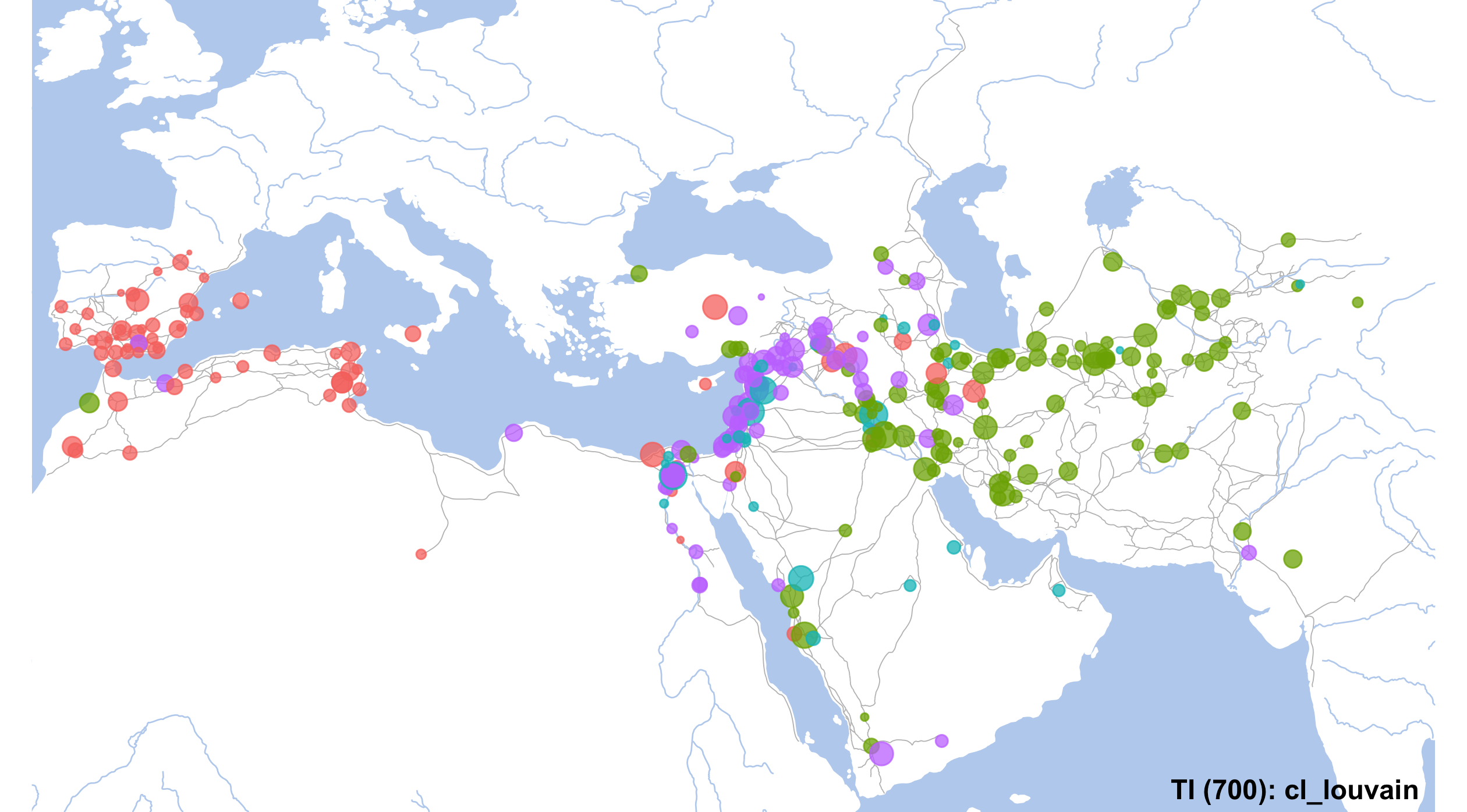

unique(NW_Final_Nodes$cl_walktrap)

## [1] "1" "3" "2" "4"

set.seed(12)

# final map
currentMap <- IslamicWorldBaseBare + 
  #geom_encircle(data=mapLayer_Filtered, s_shape=.1, expand=0.01, alpha=.15, aes(x=LON, y=LAT, col=aRegion, fill=aRegion, group=aRegion)) +
  geom_point(data=NW_Final_Nodes, aes(x=LON, y=LAT, color=cl_walktrap, size=degree), alpha=0.75) +
  annotate("text", label="TI (700): cl_walktrap", x=80, y=12.5, angle=0, hjust=1, vjust=0, size=4, col="black", alpha=1, fontface="bold") +
  coord_sf(xlim=c(min(althurayyaNodesFilt$LON)-1, max(althurayyaNodesFilt$LON)+1),
           ylim=c(min(althurayyaNodesFilt$LAT)-1, max(althurayyaNodesFilt$LAT)+1),
                 expand=FALSE) +
  scale_size_continuous(range=c(0.5,5))
  
# and saving
gt <- ggplot_gtable(ggplot_build(currentMap))
ge <- subset(gt$layout, name == "panel")
ggsave(file=paste0("./files/networks/IW_TI_000_700_cl_walktrap.png"),
       plot=grid.draw(gt[ge$t:ge$b, ge$l:ge$r]),
       dpi=300,width=8.4,height=4.65)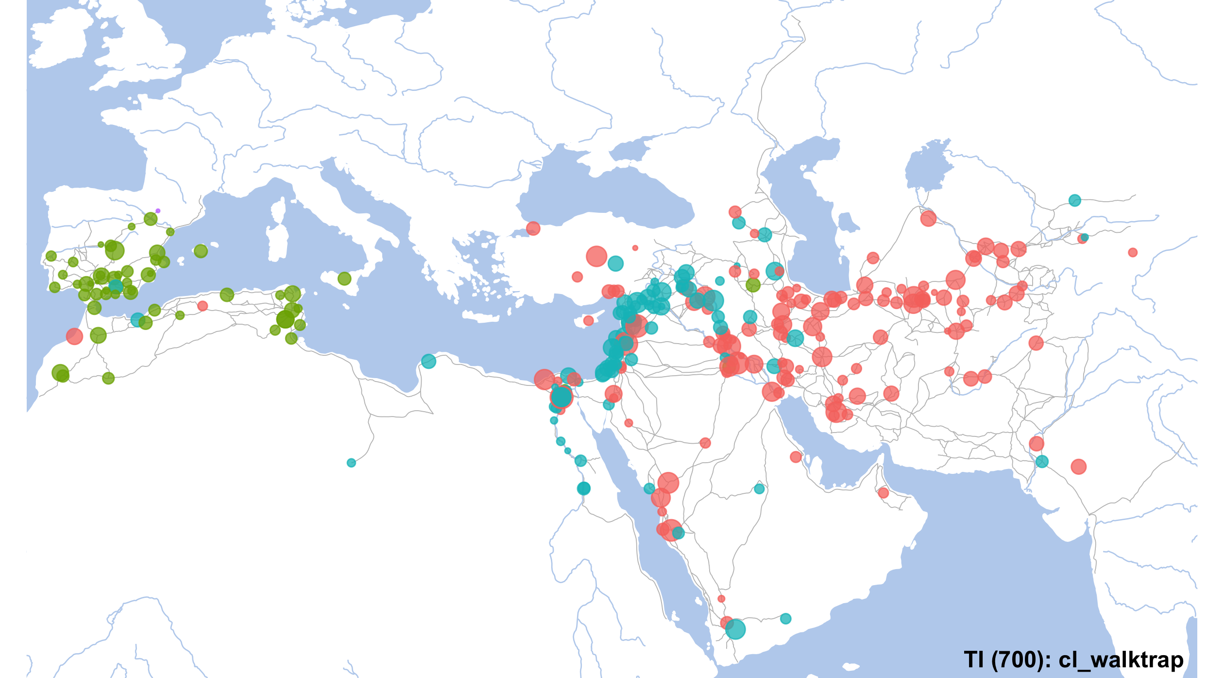

10.5 Additional Materials on Networks in R

• Katherine Ognyanova (2017-2018). Static and dynamic network visualization with R. https://kateto.net/network-visualization.

• Chapter 6 in: Arnold, Taylor, and Lauren Tilton. 2015. Humanities Data in R. New York, NY: Springer Science+Business Media.

• See also: Chapter 1 in Yunran Chen. Introduction to Network Analysis Using R (https://yunranchen.github.io/intro-net-r/index.html)

• Jesse Sadler. 2017. Introduction to Network Analysis with R: Creating static and interactive network graphs, https://www.jessesadler.com/post/network-analysis-with-r/.

• On communities:

  • http://networksciencebook.com/chapter/9.
  • https://www.r-bloggers.com/summary-of-community-detection-algorithms-in-igraph-0-6/
  • https://stackoverflow.com/questions/9471906/what-are-the-differences-between-community-detection-algorithms-in-igraph/

10.6 Homework

• A Subway Network:
  • create data for a subway system of Vienna or any other city of your choice (nodes and edges)
  • visualize the network;
  • find most important nodes (use centrality measures); visualize your results;
  • write code that finds the shortest path between any two nodes.
• Pick 3 to 5 of the above explained tasks and repeat them using different data.
  • Suggested data:
    • Orbis Data (https://purl.stanford.edu/mn425tz9757); website: https://orbis.stanford.edu/
      • ORBIS is a multimodal, seasonally variable transportation network model available at orbis.stanford.edu. The model provides for practically unlimited permutations by allowing users to limit modes, change movement cost, and adjust time of year. However, it is as a more simple network that ORBIS can be usefully integrated into other research, such as historical environmental reconstruction or agent-based modeling set in the Roman world.
    • Data of your own choice.

10.7 Submitting homework

• Homework assignment must be submitted by the beginning of the next class;
• Email your homework to the instructor as attachments.
  • In the subject of your email, please, add the following: 070184-LXX-HW-YourLastName-YourMatriculationNumber, where LXX is the numnber of the lesson for which you submit homework; YourLastName is your last name; and YourMatriculationNumber is your matriculation number.

---

1. Data on Vienna for a possible project: https://www.geschichtewiki.wien.gv.at/Personen_Zeitleiste; http://www.dasrotewien.at/↩︎