11 L11: GIS V

11.1 Interactive Maps with R

Coming soon

11.1.1 Goals

Basic approaches to interactive maps (and graphs more broadly) in R
- reference-like maps with leaflet and interactive graphs with plotly;
- semi-interactive and interactive dashboards with flexdashboard;
- interactive applications with shiny;
Hosting your results:
- githubpages on https://github.com/ for semi-interactive content;
- shinyapps on https://www.shinyapps.io/ for apps;

11.1.2 Software

R and various libraries
Data:
- Wien U-bahn: https://homepage.univie.ac.at/horst.prillinger/ubahn/english/timetables.html

# General ones 
library(tidyverse)
library(readr)
library(stringr)
library(ggplot2)

# SNA Specific
library(igraph)
library(ggraph)
library(ggrepel)
library(ggalt)

# mapping
library(rnaturalearth)
library(rnaturalearthdata)
library(grid) # grid library cuts out the plot from the graph

11.1.3 Main materials

11.1.3.1 Viennese Subway Assignment

Let’s load data. It must be prepared in such a way so that we could plot it. How should we prepare the data?

ubahnEdges <- read_delim("./data_temp/wien_data/wien_ubahn.csv", 
    ",", escape_double = FALSE, trim_ws = TRUE)
ubahnNodes <- read_delim("./data_temp/wien_data/wien_ubahn_nodes.csv", 
    ",", escape_double = FALSE, trim_ws = TRUE)

ubahnEdgesPlot <- ubahnEdges %>%
  rename(EDGELINE = LINE) %>%
  left_join(ubahnNodes, by = c("FROM"="STATION")) %>%
  rename(XFROM = XVAL, YFROM = YVAL) %>%
  left_join(ubahnNodes, by = c("TO"="STATION")) %>%
  rename(XTO = XVAL, YTO = YVAL)

ubahnNodesPlot <- ubahnNodes

These are the nodes and the edges:

head(ubahnEdges)

## # A tibble: 6 x 3
##   FROM              TO                LINE 
##   <chr>             <chr>             <chr>
## 1 Leopoldau         Großfeldsiedlung  U1   
## 2 Großfeldsiedlung  Aderklaaer Straße U1   
## 3 Aderklaaer Straße Rennbahnweg       U1   
## 4 Rennbahnweg       Kagraner Platz    U1   
## 5 Kagraner Platz    Kagran            U1   
## 6 Kagran            Alte Donau        U1

head(ubahnNodes)

## # A tibble: 6 x 4
##   STATION           LINE   XVAL  YVAL
##   <chr>             <chr> <dbl> <dbl>
## 1 Aderklaaer Straße U1      315   240
## 2 Alaudagasse       U1      220    15
## 3 Alser Straße      U6      145   175
## 4 Alte Donau        U1      285   210
## 5 Alterlaa          U6      130    40
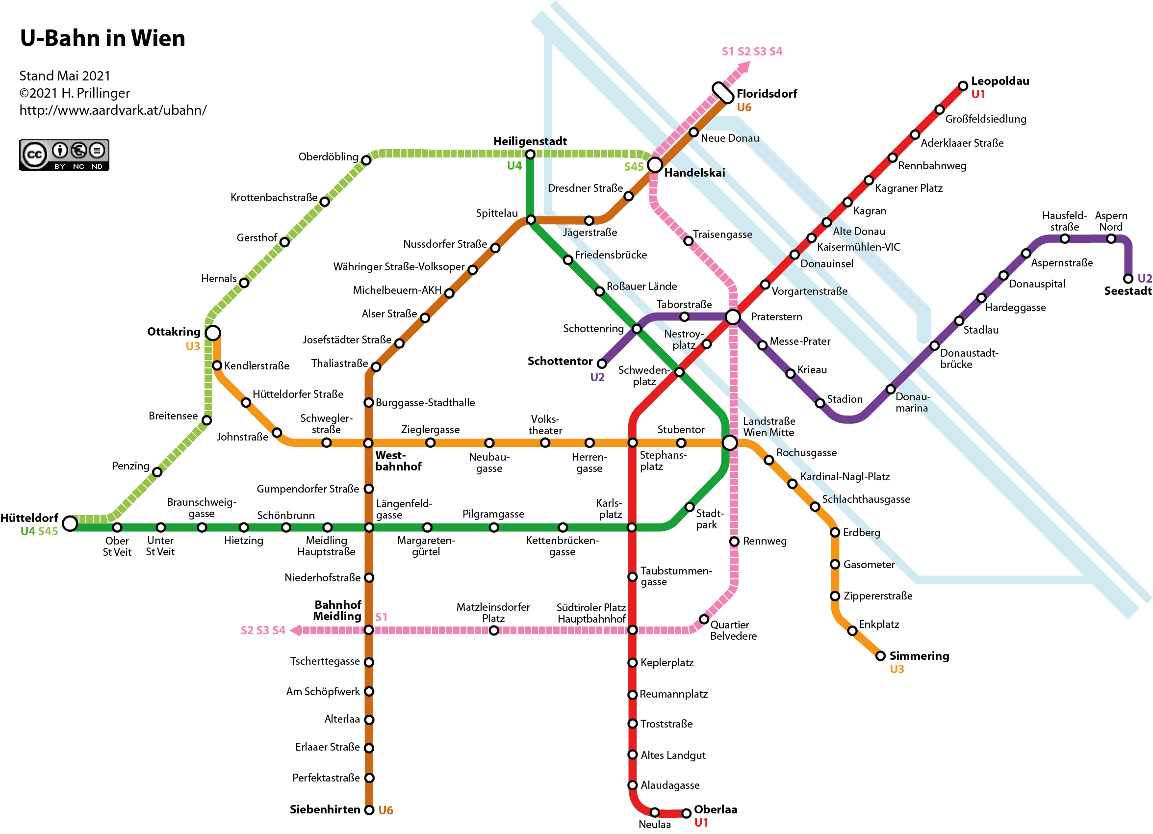
## 6 Altes Landgut     U1      220    25

You can see XVAL and YVAL columns: they are coordinates of our stations (well, sort of). What we want to do is a cartogram (i.e., not a proper map) where positions of points vis-à-vis each other points to their relative positions in real space without faithfully representing it—like all subway schemes.

How to get/collect these “coordinates?” You can use most image editors. A screenshot below shows the Vienna subway cartogram (the one from above) opened in Gimp (https://www.gimp.org/), a free text editor for most operating systems. When you hover your mouse over any point, the program will show the position of that point in the lower left corner—those are X and Y values, which can be used as “coordinates” (they can be in pixels, in cantimeters, in millimeters — it does not matter as they will work pretty much the same in ggplot). Collecting those might take some time, of course.

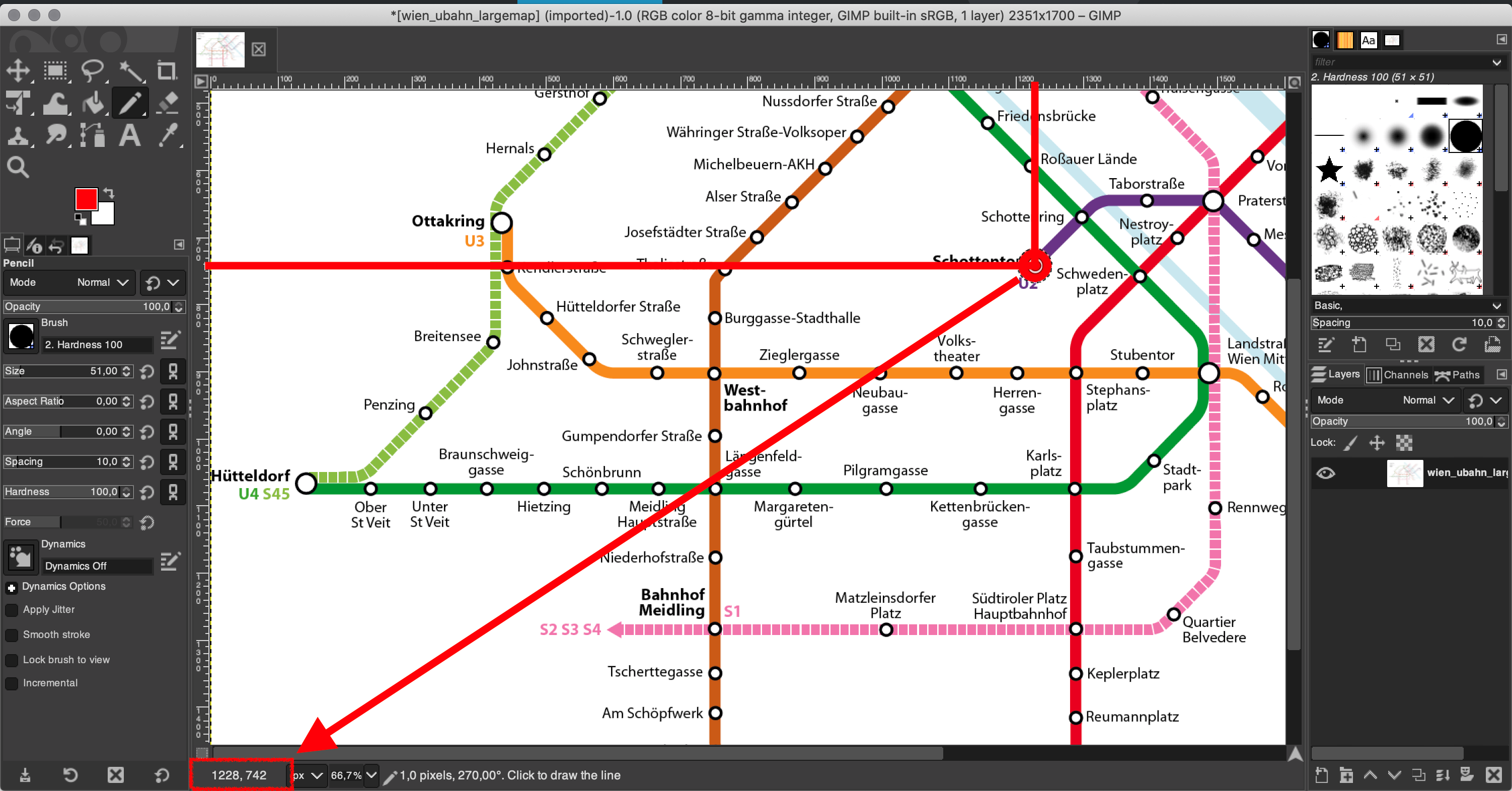
Let’s plot the U-bahn map, which we will use as our base layer:

colorVals <- c("U1" = "red", "U2" = "darkviolet",  "U3" = "goldenrod3",
               "U4" = "darkgreen", "U6" = "darkorange4")

ggplot() +
  geom_segment(data=ubahnEdgesPlot, aes(x=XFROM, y=YFROM, xend=XTO, yend=YTO, color=EDGELINE), lwd=3) +
  geom_point(data=ubahnNodesPlot, aes(x=XVAL, y=YVAL), color="black", size=3) +
  geom_point(data=ubahnNodesPlot, aes(x=XVAL, y=YVAL), color="white", size=2) +
  geom_text_repel(data=ubahnNodesPlot, aes(x=XVAL, y=YVAL, label=STATION), color="black", size=2, max.overlaps=100) +
  theme_void() +
  theme(legend.position = "none") +
  scale_color_manual(values = colorVals, aesthetics = c("color"))

These are the names of stations:

ubahnNodes$STATION

##  [1] "Aderklaaer Straße"             "Alaudagasse"                  
##  [3] "Alser Straße"                  "Alte Donau"                   
##  [5] "Alterlaa"                      "Altes Landgut"                
##  [7] "Am Schöpfwerk"                 "Aspern Nord"                  
##  [9] "Aspernstraße"                  "Braunschweiggasse"            
## [11] "Burggasse-Stadthalle"          "Donauinsel"                   
## [13] "Donaumarina"                   "Donauspital"                  
## [15] "Donaustadtbrücke"              "Dresdner Straße"              
## [17] "Enkplatz"                      "Erdberg"                      
## [19] "Erlaaer Straße"                "Floridsdorf"                  
## [21] "Friedensbrücke"                "Gasometer"                    
## [23] "Großfeldsiedlung"              "Gumpendorfer Straße"          
## [25] "Handelskai"                    "Hardeggasse"                  
## [27] "Hausfeldstraße"                "Heiligenstadt"                
## [29] "Herrengasse"                   "Hietzing"                     
## [31] "Hütteldorf"                    "Hütteldorfer Strasse"         
## [33] "Jägerstraße"                   "Johnstrasse"                  
## [35] "Josefstädter Straße"           "Kagran"                       
## [37] "Kagraner Platz"                "Kaisermühlen-VIC"             
## [39] "Kardinal-Nagl-Platz"           "Karlsplatz"                   
## [41] "Kendlerstrasse"                "Keplerplatz"                  
## [43] "Kettenbrückengasse"            "Krieau"                       
## [45] "Landstrasse"                   "Längenfeldgasse"              
## [47] "Leopoldau"                     "Margaretengürtel"             
## [49] "Meidling Hauptstr."            "Messe-Prater"                 
## [51] "Michelbeuern-AKH"              "Museumsquartier"              
## [53] "Nestroyplatz"                  "Neubaugasse"                  
## [55] "Neue Donau"                    "Neulaa"                       
## [57] "Niederhofstraße"               "Nußdorfer Straße"             
## [59] "Ober St. Veit"                 "Oberlaa"                      
## [61] "Ottakring"                     "Perfektastraße"               
## [63] "Philadelphiabrücke"            "Pilgramgasse"                 
## [65] "Praterstern"                   "Rathaus"                      
## [67] "Rennbahnweg"                   "Reumannplatz"                 
## [69] "Rochusgasse"                   "Rossauer Lände"               
## [71] "Schlachthausgasse"             "Schönbrunn"                   
## [73] "Schottenring"                  "Schottentor"                  
## [75] "Schwedenplatz"                 "Schweglerstrasse"             
## [77] "Seestadt"                      "Siebenhirten"                 
## [79] "Simmering"                     "Spittelau"                    
## [81] "Stadion"                       "Stadlau"                      
## [83] "Stadtpark"                     "Stephansplatz"                
## [85] "Stubentor"                     "Südtiroler Platz-Hauptbahnhof"
## [87] "Taborstraße"                   "Taubstummengasse"             
## [89] "Thaliastraße"                  "Troststraße"                  
## [91] "Tscherttegasse"                "Unter St. Veit"               
## [93] "Volkstheater"                  "Vorgartenstraße"              
## [95] "Währinger Straße-Volksoper"    "Westbahnhof"                  
## [97] "Zieglergasse"                  "Zippererstrasse"

Now, we need to run the search for the shortest path from station A to station B, and then graph it.

ubahnNetwork <- graph_from_data_frame(d=ubahnEdges, vertices=ubahnNodes, directed=FALSE)
shortest_path <- shortest_paths(ubahnNetwork, from = "Zieglergasse", to = "Taborstraße")$vpath

shortest_path <- names(unlist(shortest_path))
shortest_path <- tibble(ID = shortest_path) %>%
  left_join(ubahnNodes, by = c("ID" = "STATION"))

ggplot() +
  geom_segment(data=ubahnEdgesPlot, aes(x=XFROM, y=YFROM, xend=XTO, yend=YTO), color="grey", lwd=3) +
  geom_path(data = shortest_path, aes(x=XVAL, y=YVAL), col="red", lwd=4) + 
  geom_point(data=ubahnNodesPlot, aes(x=XVAL, y=YVAL), color="black", size=3) +
  geom_point(data=ubahnNodesPlot, aes(x=XVAL, y=YVAL), color="white", size=2) +
  geom_text_repel(data=ubahnNodesPlot, aes(x=XVAL, y=YVAL, label=STATION), color="black", size=2, max.overlaps=100) +
  theme_void() +
  theme(legend.position = "none")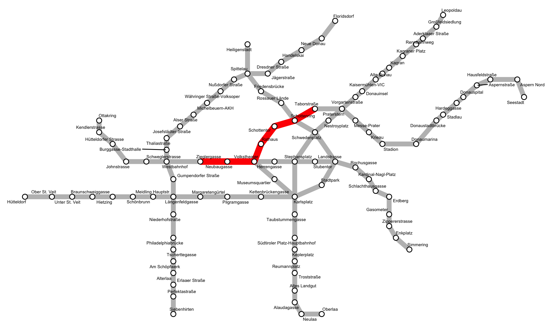

ubahnNetwork <- graph_from_data_frame(d=ubahnEdges, vertices=ubahnNodes, directed=FALSE)
shortest_path <- shortest_paths(ubahnNetwork, from = "Seestadt", to = "Westbahnhof")$vpath

shortest_path <- names(unlist(shortest_path))
shortest_path <- tibble(ID = shortest_path) %>%
  left_join(ubahnNodes, by = c("ID" = "STATION"))

ggplot() +
  geom_segment(data=ubahnEdgesPlot, aes(x=XFROM, y=YFROM, xend=XTO, yend=YTO), color="grey", lwd=3) +
  geom_path(data = shortest_path, aes(x=XVAL, y=YVAL), col="red", lwd=4) + 
  geom_point(data=ubahnNodesPlot, aes(x=XVAL, y=YVAL), color="black", size=3) +
  geom_point(data=ubahnNodesPlot, aes(x=XVAL, y=YVAL), color="white", size=2) +
  geom_text_repel(data=ubahnNodesPlot, aes(x=XVAL, y=YVAL, label=STATION), color="black", size=2, max.overlaps=100) +
  theme_void() +
  theme(legend.position = "none")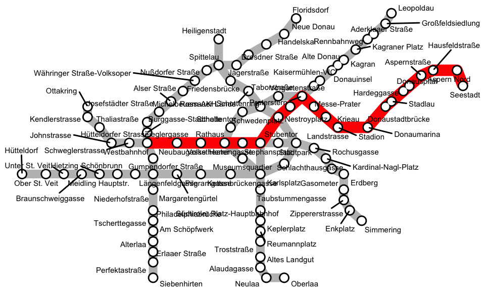

11.1.4 Interactive Content with `leaflet`

With Leaflet library (which connects into Leaflet Javascript library, https://leafletjs.com/) we can create rather robust maps of reference type. That is to say, Leaflet does not provide any analytical fucntionality, but allows to put information on a map that can then be used as a reference of some kind. It is quite simple, but it does get the job done in many cases.

# LIBRARIES
library(leaflet)

## Warning: package 'leaflet' was built under R version 4.0.2

iwSettlements <- read_delim("./data_temp/althurayya/settlements.csv",
                            "\t", escape_double = FALSE, trim_ws = TRUE) %>%
  separate(col=coordinates, into=c("l", "lon", "lat", "r"), sep="([\\[, \\]]+)") %>%
  select(settlement_id, names_eng_translit, region_URI, top_type, lon, lat) %>%
  mutate(lon = as.numeric(lon), lat = as.numeric(lat))

## Parsed with column specification:
## cols(
##   settlement_id = col_character(),
##   languages = col_character(),
##   names_ara_common = col_character(),
##   names_ara_common_other = col_character(),
##   names_ara_search = col_character(),
##   names_ara_translit = col_logical(),
##   names_ara_translit_other = col_logical(),
##   names_eng_common = col_character(),
##   names_eng_common_other = col_character(),
##   names_eng_search = col_character(),
##   names_eng_translit = col_character(),
##   names_eng_translit_other = col_character(),
##   region_URI = col_character(),
##   source = col_character(),
##   top_type = col_character(),
##   coordinates = col_character()
## )

iwRoutes <- read_delim("./data_temp/althurayya/routes.csv", 
    "\t", escape_double = FALSE, trim_ws = TRUE)

## Parsed with column specification:
## cols(
##   route_id = col_character(),
##   sToponym = col_character(),
##   sToponym_type = col_character(),
##   eToponym = col_character(),
##   eToponym_type = col_character(),
##   terrain = col_character(),
##   safety = col_character(),
##   coordinates = col_character(),
##   meter = col_double()
## )

Leaflet does not automatically assign colors from categorical data like ggplot, so we need to perform some manipulations with our data:

assign colors to different provinces (so that each province is highlighted with its own color);
assign sizes to points based on their types;
generate a pop up message

# additional data for regions -- simply loading
iwRegions <- read_delim("./data_temp/althurayya/regions.csv",
                            "\t", escape_double = FALSE, trim_ws = TRUE)

## Parsed with column specification:
## cols(
##   region_URI = col_character(),
##   region_code = col_character(),
##   region_color = col_character(),
##   region_name = col_character()
## )

# additional data for sizing --- can be formed in a CSV, or generated like shown below
types <- tibble(top_type = unique(iwSettlements$top_type),
                size = c(5, 3, 0, 2, 0, 1, 0, 4, 0, 0))

# now let's add everything with left_join, and then format a pop-up message
iwSettlementsMOD <- iwSettlements %>%
  left_join(iwRegions, by = c("region_URI")) %>%
  left_join(types, by = c("top_type")) %>%
  mutate(popup = paste0("<b>", names_eng_translit, "</b> is one of ", top_type,
                        ". It is located in the province of ", region_name, " (", 
                        lon, ", ", lat, ").")) %>%
  filter(top_type %in% c("metropoles", "capitals", "towns", "villages", "waystations"))

iwSettlementsMOD

## # A tibble: 1,812 x 11
##    settlement_id names_eng_trans… region_URI top_type    lon   lat region_code
##    <chr>         <chr>            <chr>      <chr>     <dbl> <dbl> <chr>      
##  1 QAHIRA_312E3… al-Qāhiraŧ       Misr_RE    metropo… 31.2    30.0 Egypt      
##  2 IRBIL_440E36… Irbīl            Aqur_RE    towns    44.0    36.2 Aqur       
##  3 DANIYA_001E3… Dāniyaŧ          Andalus_RE towns     0.105  38.8 Andalus    
##  4 WASHQA_003W4… Wašqaŧ           Andalus_RE towns    -0.354  42.2 Andalus    
##  5 BALANSIYYA_0… Balansiyyaŧ      Andalus_RE towns    -0.415  39.4 Andalus    
##  6 SHAQR_004W39… al-Šaqr          Andalus_RE villages -0.437  39.2 Andalus    
##  7 QANT_004W383… Qānt             Andalus_RE towns    -0.471  38.3 Andalus    
##  8 SHATIBA_005W… Šātibaŧ          Andalus_RE towns    -0.523  39.0 Andalus    
##  9 SARAQUSA_009… Saraqūsaŧ        Andalus_RE towns    -0.929  41.6 Andalus    
## 10 QARTAJANNA_0… Qarṭāǧannaŧ      Andalus_RE villages -0.983  37.6 Andalus    
## # … with 1,802 more rows, and 4 more variables: region_color <chr>,
## #   region_name <chr>, size <dbl>, popup <chr>

Now we can combine everything:

Base groups: there are plently of base map layers: http://leaflet-extras.github.io/leaflet-providers/preview/index.html
Overlay groups: this is where you add your data; you can add a legend as well;
Layer control: you can use it for switching layers of your data on and off;
check official documentation for additional options: https://rstudio.github.io/leaflet/

m <- leaflet(iwSettlementsMOD) %>%
  # Base groups
  addProviderTiles(providers$Esri.WorldPhysical, group = "World Physical (ESRI)") %>%
  addProviderTiles(providers$Esri.WorldTerrain, group = "World Terrain (ESRI)") %>%
  addProviderTiles(providers$Esri.WorldImagery, group = "World Imagery (ESRI)") %>%
  addProviderTiles(providers$Esri.WorldShadedRelief, group = "World ShadowRelief (ESRI)") %>%
  addProviderTiles(providers$Thunderforest.Pioneer, group = "Thunderforest Pioneer") %>%
  addProviderTiles(providers$Stamen.Watercolor, group = "Watercolor") %>%
  addProviderTiles(providers$Stamen.Toner, group = "Toner") %>%
  addProviderTiles(providers$Stamen.TonerLite, group = "Toner Lite") %>%
  addProviderTiles(providers$CartoDB.DarkMatter, group = "Dark Matter") %>%
  setView(32, 32, zoom = 5) %>%
  # Overlay groups
  addCircles(~lon, ~lat, popup=~popup, weight = ~size*2, radius=~size*10, 
                 color=~region_color, stroke = TRUE, fillOpacity = 1, group = "All regions")  %>%
  addLabelOnlyMarkers(~lon, ~lat, label=~names_eng_translit, labelOptions = labelOptions(noHide = F)) %>%
  addLegend("bottomleft", colors = iwRegions$region_color,
            labels = iwRegions$region_name, title  = "Islamic World (11th Century)") %>%
  # Layers control
  addLayersControl(
    baseGroups = c("World Physical (ESRI)", "World Terrain (ESRI)", "World Imagery (ESRI)", "World ShadowRelief (ESRI)",
                   "Toner", "Toner Lite", "Dark Matter", "Watercolor",
                   "Thunderforest Pioneer"),
    overlayGroups = c(#"al-ʿIrāq (Iraq)",
                      #"Labels",
                      "All regions"),
    options = layersControlOptions(collapsed = FALSE)
  )

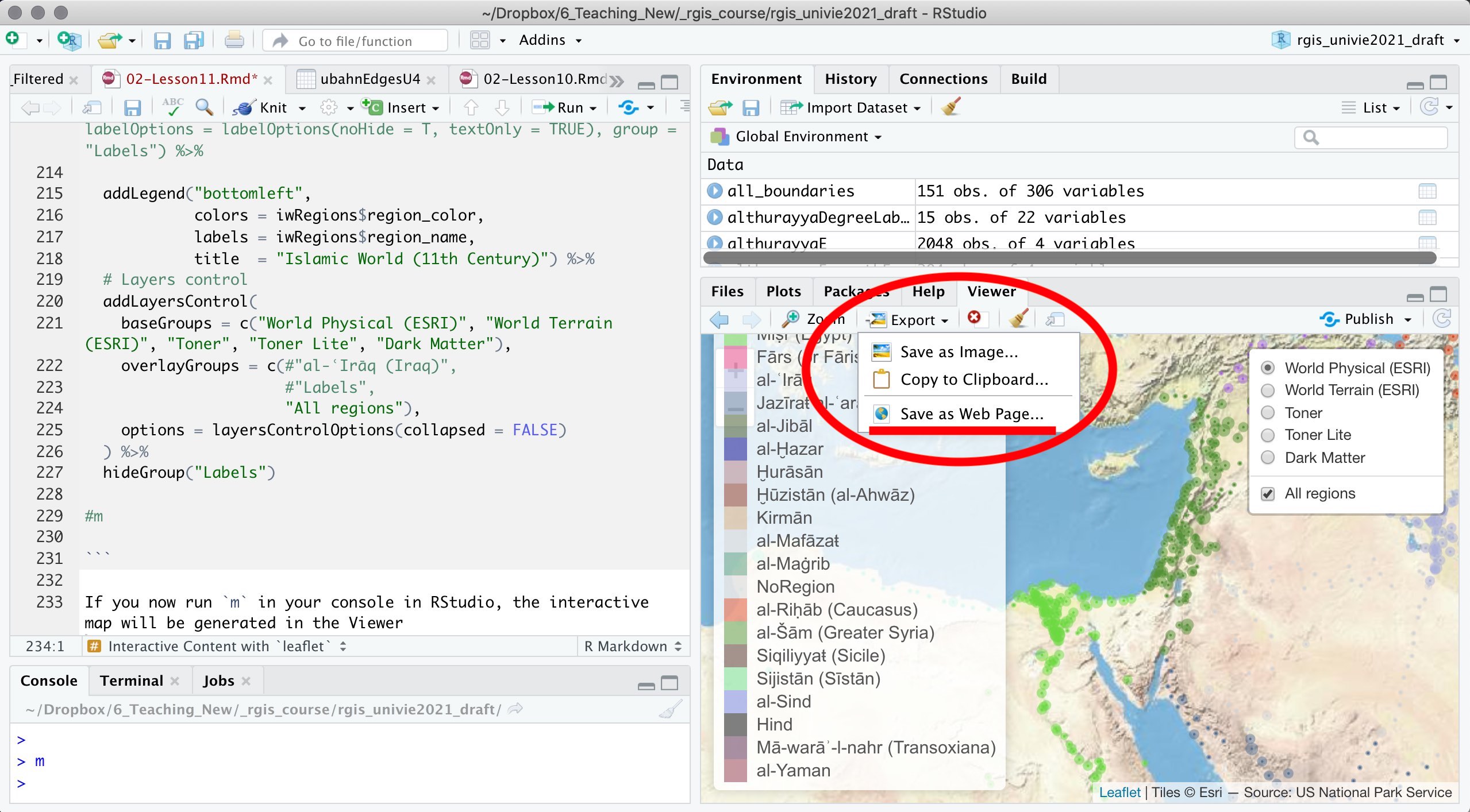
#m

If you now run m in your console in RStudio, the interactive map will be generated and shown in the Viewer. You can save this map now as an HTML page and then use it however you find necessary. (Export > Save as Web Page…) You can upload this HTML file to your website or show it from your computer — in any browser (well, in most browsers; internet connection will be necessary for loading the base map layers). Here is the link to the map.

11.1.5 Simple summaries of your data with `flexdashboard`

flexdashboard is aimed at delivering primarily semi-interactive summaries of your data. Semi- here means that the interactivity is highly limited and is provided primarily through some HTML+Javascript elements. Nothing that requires to run R code can be incorporated into these semi-interactive summaries. flexdashboard creates “static” HTML pages, which can be open in most browsers and can be hosted on any website. (NB: flexdashboard may use some shiny components—see the next section—in which case an RStudio Shiny Server will be necessary to run your dashboard.)

easy and fast to create with Rmarkdown;
usually, the “end product” fits into a single file (code and data together);
created for web (mobile including);
for simple summaries of your data;
for small amounts of data; for data that can be shared with others;
can work on any website: no special features necessary;
SIMPLE EXAMPLE: Empty Template
COMPLEX EXAMPLE: Islamic World Geographical Data

Note: I am not including any code from these flexdashboards, because you can get it directly from the examples.

Recommended: RStudio has multiple learning materials on their products:

Introducing flexdashboards by Garrett Grolemund (https://www.rstudio.com/resources/webinars/introducing-flexdashboards/)
Documentation (with lots of usable examples): https://pkgs.rstudio.com/flexdashboard/

11.1.6 Dynamic apps with `shiny`

shiny is another library (+ the whole ecosystem) that allows one to convert any code that you write in R into an interactive app. These are a bit trickier to write, but allow you to do much more — practically anything that you can do with R. These are also tricker to host: you (and others) can run these apps on their local machines (R, RStudio and all the necessary libraries must be installed), or you can host is on a server which runs RStudio Shiny Server (https://www.shinyapps.io/ is offered by RStudio as a fremium option where you can host your apps)

uses its own syntax (R + shiny); a certain learning curve;
the “end product” is a package of files (code and data separately);
for complex functionality;
for larger amounts of data; for data that must not be shared with end users;
requires a special RStudio Shiny Server to run;

11.1.6.1 Examples

SIMPLE EXAMPLE: Vienna Subway
you can download the entire app from here: Vienna Subway App

The code for this app looks as follows. THere are three parts

######################################################################################################
# PART I :: LIBRARIES & DATA #########################################################################
######################################################################################################

library(shiny)
library(tidyverse)
library(readr)
library(stringr)
library(ggplot2)
library(igraph)
library(ggrepel)

# LOAD AND PREPARE DATA

ubahnEdges <- read_delim("wien_ubahn.csv", ",", escape_double = FALSE, trim_ws = TRUE)
ubahnNodes <- read_delim("wien_ubahn_nodes.csv", ",", escape_double = FALSE, trim_ws = TRUE)

stations <- ubahnNodes$STATION # for the drop down list of stations

ubahnEdgesPlot <- ubahnEdges %>%
  rename(EDGELINE = LINE) %>%
  left_join(ubahnNodes, by = c("FROM"="STATION")) %>% rename(XFROM = XVAL, YFROM = YVAL) %>%
  left_join(ubahnNodes, by = c("TO"="STATION")) %>% rename(XTO = XVAL, YTO = YVAL)

ubahnNodesPlot <- ubahnNodes
ubahnNetwork <- graph_from_data_frame(d=ubahnEdges, vertices=ubahnNodes, directed=FALSE)

######################################################################################################
# PART II :: FUNCTION THAT CALCULATES THE PATH AND GRAPHS IT  ########################################
######################################################################################################

subwayPath <- function(departure, arrival){
  shortest_path <- shortest_paths(ubahnNetwork, from = departure, to = arrival)$vpath
  shortest_path <- names(unlist(shortest_path))
  shortest_path <- tibble(ID = shortest_path) %>%
    left_join(ubahnNodes, by = c("ID" = "STATION"))
  
  ggplot() +
    geom_segment(data=ubahnEdgesPlot, aes(x=XFROM, y=YFROM, xend=XTO, yend=YTO), color="grey", lwd=3) +
    geom_path(data = shortest_path, aes(x=XVAL, y=YVAL), col="red", lwd=4) + 
    geom_point(data=ubahnNodesPlot, aes(x=XVAL, y=YVAL), color="black", size=3) +
    geom_point(data=ubahnNodesPlot, aes(x=XVAL, y=YVAL), color="white", size=2) +
    geom_text_repel(data=ubahnNodesPlot, aes(x=XVAL, y=YVAL, label=STATION), color="black", size=2, max.overlaps=100) +
    theme_void() +
    theme(legend.position = "none")
}

######################################################################################################
# PART III :: THE APP ITSELF  ########################################################################
######################################################################################################

# Define UI ----
ui <- fluidPage(
  titlePanel("Vienna Subway"),
  textOutput("itinerary"), # output$itinerary
  plotOutput("shortestPath", width="100%"), # output$shortestPath

  fluidRow(
    column(width = 3, selectInput("from_station", "From", stations)),
    column(width = 3, selectInput("to_station", "To", stations))
  )
)

# Define server logic ----
server <- function(input, output) {
  output$itinerary <- renderText({paste0("Traveling from ", input$from_station, " to ", input$to_station)})
  output$shortestPath <- renderPlot({subwayPath(input$from_station, input$to_station)})
}

# Run the app ----
shinyApp(ui = ui, server = server)

Parts I and II should be very familar to you by now. Part I simply loads all the libraries and then loads and prepares all the necessary data. Part II should be rather clear as well, except for, perhaps, the function part. We have briefly touched upon creating our own functions before, but have not used them much. The only thing to pay attention to here is that subwayPath is a small program of sorts that takes two stations as its arguments and draws the shortest path between them.

Part III is a totally new thing. This is where we create the app itself and define all the things that appear in the user interface (ui) and all the things that are done by R under the hood (server). Let’s take a closer look. (A bit of a confusing thing is that variables sometimes appear as variables (input$itinerary), and sometimes — as strings (“itinerary”), but this should become clear with some practice.)

ui is the variable for our interface:
- everything here is inside the function fluidPage, which is responsible for creating the main interface (elements are connected with commas!);
  - titlePanel() creates the main header;
  - textOutput() prints out “itinerary,” which is takes from the variable output$itinerary that is [re]created in the server part;
  - plotOutput() plots out a graph that is [re]created in the server part;
  - fluidRow() creates an table, where we can add columns (column(); width determines the relative width of the column, which is measured in 12 parts — so 3 is a quarter of the window width)
    - inside the column() function we create a drop down menu:
      - “from_station” becomes variable input$from_station in the server part;
      - stations gives us the list of values for the drop down menu;
    - (the same is for the “to_station” line.)
server is our main functionality:
- note that the actual R code is between curly brakets ({...}); on the outside of the R code there are shiny rendering functions;
- output$itinerary:
  - here everything is rather simple: we take variables selected in the ui — input$from_station and input$to_station — and paste0 them together into a readable line of text; output$itinerary becomes available to the ui for printing out with textOutput("itinerary");
- output$shortestPath:
  - here we call our function subwayPath() that takes departure and arrival as its arguments; we give it input$from_station and input$to_station which has been selected in the ui; then renderPlot() generates a graph which is made available to the ui for plotting wth plotOutput("shortestPath")
shinyApp(ui = ui, server = server) activates our ui and our server.