11 Lesson 11: Mapping Data (using tagged data)
11.1 Preparing and Modeling Geospatial Data
In a similar manner we can also graph geographical data — in combination with the temporary dimension. For this, however, we need to think through what kind of insight we can possibly get from geospatial data and how it should be prepared for mapping.
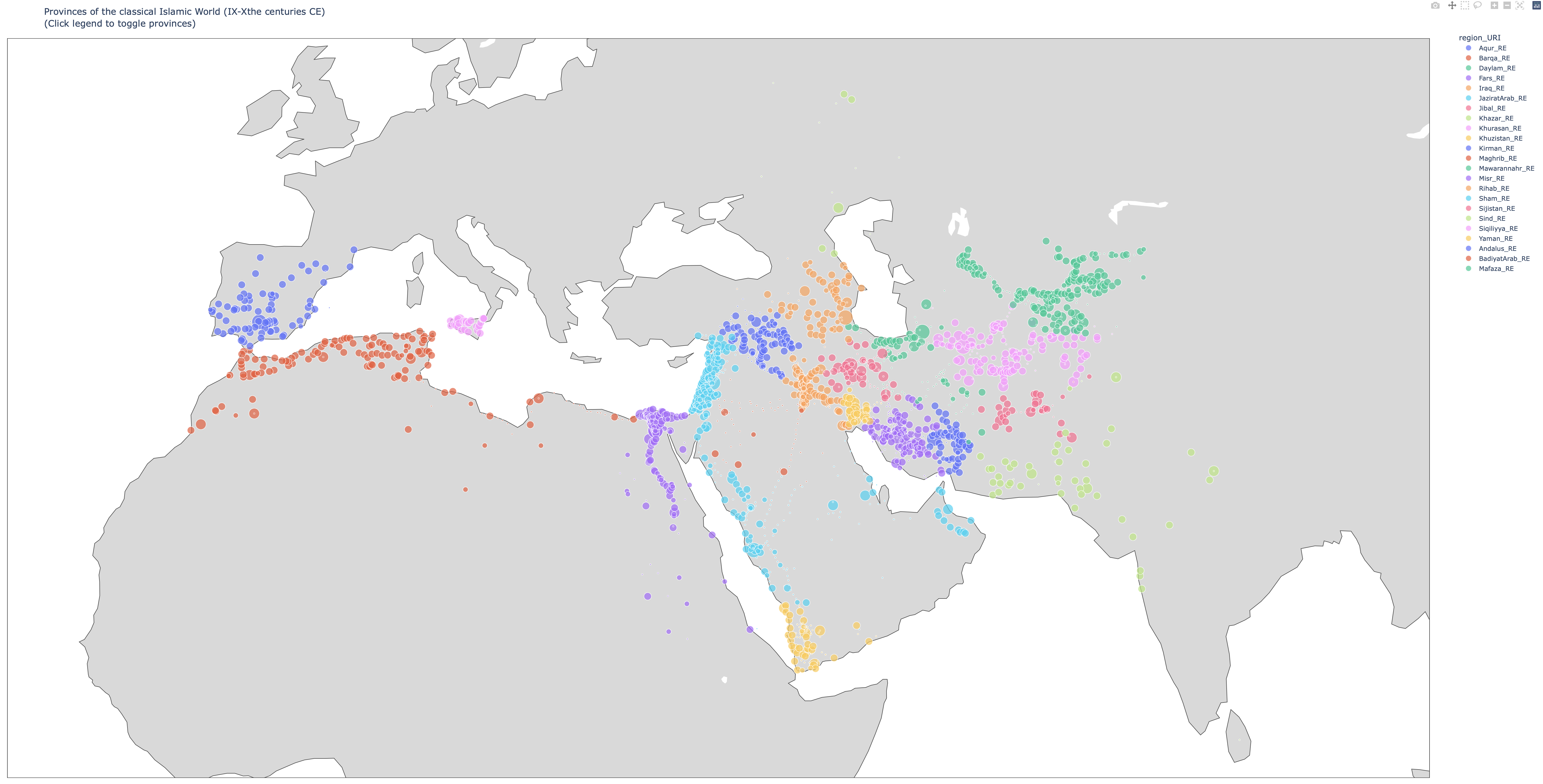
Let’s start with a simple task: we will map the geospatial data from one of the previous lessons: settlements from the al-Thurayya Gazetteer. Below is the code that produces an interactive map. (Note: it is possible to use matplotlib for mapping, but installation of needed components has become rather complicated recently, so we will proceed with a different library, plotly, which produced web-oriented maps.)
import plotly.express as px
import pandas as pd

althurayyaFile = "settlements.csv"

df = pd.read_csv(althurayyaFile, sep="\t", header=0)
print(df)

fig = px.scatter_geo(df, lon='lon', lat='lat', color="region_URI",
                     hover_name="names_eng_translit", size=df["top_size"]*df["top_size"],
                     projection="natural earth", fitbounds='locations')

fig.update_layout(
    title_text='Provinces of the classical Islamic World (IX-Xthe centuries CE)<br>(Click legend to toggle provinces)',
    showlegend=True,
    geo=dict(
        scope='world',
        landcolor='rgb(250, 250, 250)',
    )
)

fig.show()

# the following line will save the graph into an html file
fig.write_html("althurayya.html")
We can get the following map (for an interactive map, try this link):
 We can also map our geographical data dynamically, if we want to highlight its chronological dimension. Below is the example of the growth of US cities. Click here for the interactive graph.
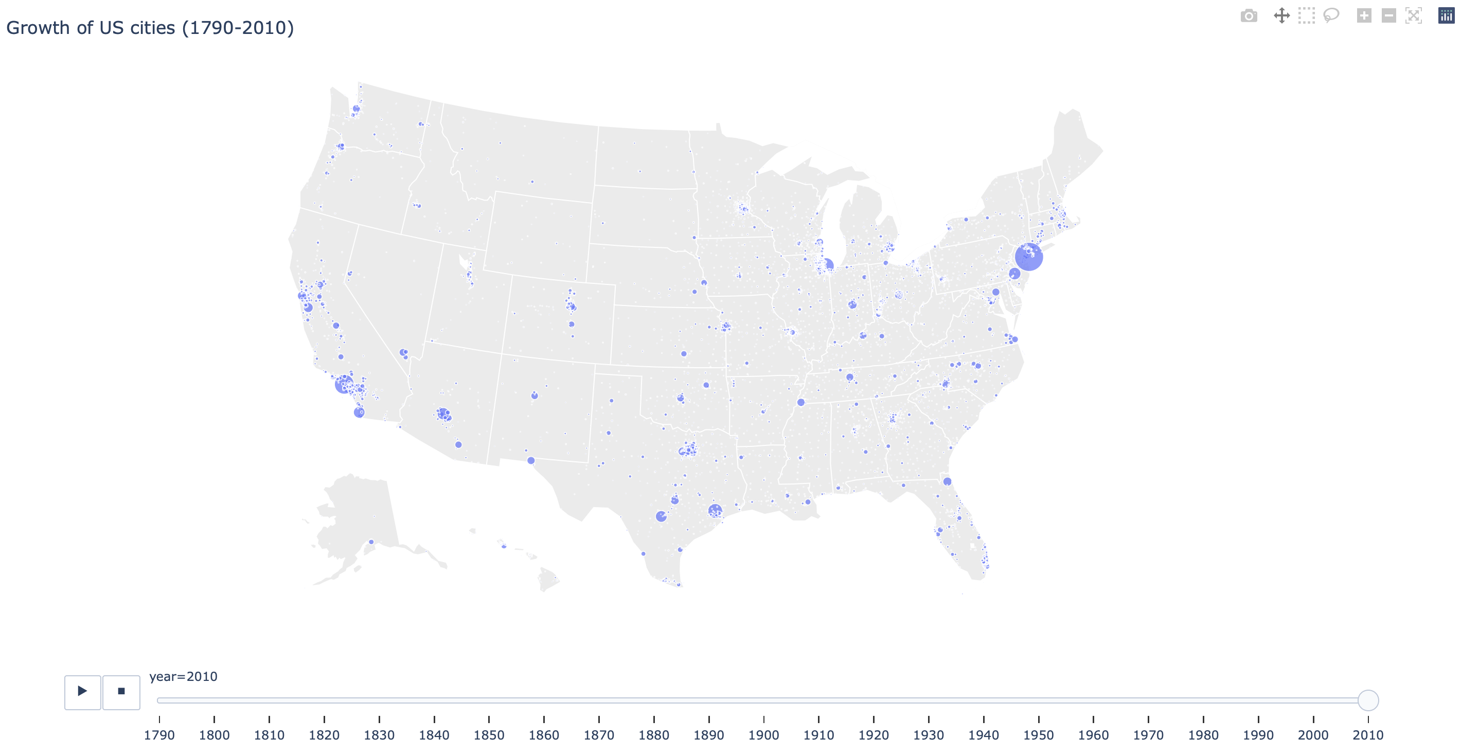 The following code is used to produce the visualization above. Use this as a starting point for mapping data from the Dispatch. You can download the
 us_cities_pop.csv from here. One thing to keep in mind, the chronological data must be passed to the function as string, not as date (that is why there is no conversion to the date format in the code below).
import plotly.express as px
import pandas as pd
import re

us_cities_data = "us_cities_pop.csv"
usCities = pd.read_csv(us_cities_data, sep=",", header=0)

# plot places
placesAll = usCities[['year', 'cityst', 'population', 'lat', 'lon']]
print(placesAll)

fig = px.scatter_geo(placesAll, lon='lon', lat='lat',
                     hover_name="cityst",
                     animation_frame="year",
                     size='population')

fig.update_layout(
    title_text='Growth of US cities (1790-2010)',
    showlegend=True,
    geo=dict(
        scope='usa',
        landcolor='rgb(235, 235, 235)',
    )
)

fig.show()
fig.write_html("us_cities_pop.html")
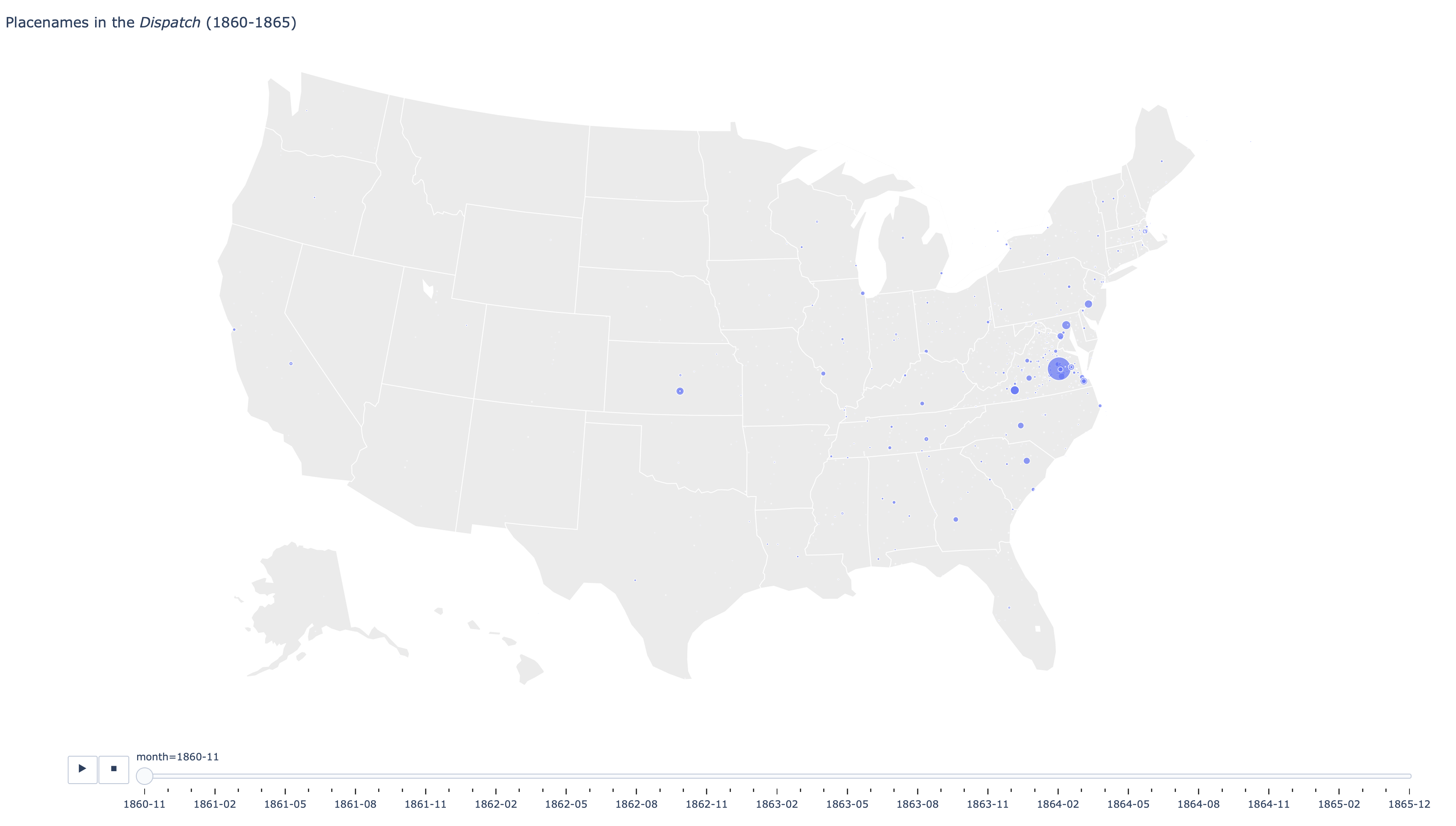
Now, let’s get back to our Dispatch data. We have placenames tagged — and we already have the data ready for processing. We can focus on a specific period of time (by filtering our data, including only dates that we are interested in). Then we need to calculate frequencies of mentions of placenames — we can use these values to size dots on the final map. Unfortunately, a very important element is missing — as you recall, our data does not have any coordinates. Luckily, we have unique identifiers from the Getty Thesaurus of Geographical Names. What we can do is to extract coordinates from the Thesaurus and connect them to corresponding placenames in our data.
- Getty Thesaurus is available for download here: http://tgndownloads.getty.edu/ and here: http://vocab.getty.edu/dataset/tgn/
- You can download
explicit.zipfrom http://vocab.getty.edu/dataset/tgn/ - There is a file
TGNOut_Coordinates.ntwith coordinates. You will need to write a script to extract coordinates from this file in order to use them. I suggest you convert this file into a usable CSV/TSV (the format isN-triples).
11.1.1 Triples (N-triples)
What are triples? This is one of the most robust formats that can describe any kind of data. The main idea is that every triple is expressed through the structure subject-predicate-object. There are multiple formats for expressing triples (for example, RDF, N-Triples, etc.) (more details…).
Let’s take a look at the following example from TGNOut_Coordinates.nt. There are three triples (N-triples) which together describe a specific object (which in our data would look like tgn,1000007).
<http://vocab.getty.edu/tgn/1000007-geometry> <http://www.w3.org/1999/02/22-rdf-syntax-ns#type> <http://schema.org/GeoCoordinates> .
<http://vocab.getty.edu/tgn/1000007-geometry> <http://schema.org/latitude> "-83.843"^^<http://www.w3.org/2001/XMLSchema#decimal> .
<http://vocab.getty.edu/tgn/1000007-geometry> <http://schema.org/longitude> "65.725"^^<http://www.w3.org/2001/XMLSchema#decimal> .
Each triple is stored on a separate line, ending with a period (“.”). Elements of each triple are separated with spaces. Each triple has the same structure—subject-predicate-object—and can be read as follows:
- Triple 1: entity
tgn,1000007has (expressed in a particular manner) geographical coordinates; - Triple 2: entity
tgn,1000007has decimal latitude-83.843; - Triple 3: entity
tgn,1000007has decimal longitude65.725;
You should have no problems writing a script that converts this data into a CSV with the structure: ID, lon, and lat. (Technically, you can also store these triples in a CSV/TSV format, but that would require additional conversion later.)
If you are not up to this challenge, you can use the CSV file that I have already prepared, to make your life a bit easier: TGNOut_Coordinates.csv.zip
If everything done correctly, the final map may look like what you see below. The complete interactive map can be found here.):
Last but not least, we may get interesting maps if we map places that co-occur with some specific names. An example of Gen. Sherman and Atlanta could be quite interesting (we have seen the graphs in the previous lesson), although in such cases a chronological graph of mentions of Atlanta—only in articles where Gen. Sherman is mentioned—may be a more clear option (see the preceding lesson). Please, try to code a solution that will do one or the other.
11.2 Homework
Graph geographical data from the Dispatch. Experiment with different periods and different selections of placenames (for example, Richmond and Virginia will be the most frequently mentioned placenames—because the newspaper was published in Richmond, Virginia; this would mean that these two places will overshadow all other places.)
- Suggestions:
- you can create a separate data file that only has placenames (
articleID,date,placename,lat,lon) - you can map places in a more complex manner. For example, map only placenames that are mentioned in the same articles as, say, General Sherman. In this case we may expect the maps to reflect his campaign through Georgia and the Carolinas (or, more precisely, the Dispatch’s coverage of Gen. Sherman’s campaign).
- for interactive maps, you can use
Plotlylibrary: https://plotly.com/python/bubble-maps/.
- you can create a separate data file that only has placenames (
- Suggestions:
Finish the assigned task;
Annotate your script (i.e., add comment to every line of code describing what is happening there);
Additional materials:
- Interactive maps with
Plotly: https://plotly.com/python/bubble-maps/; - Basemap Matplotlib Toolkit: Plotting data on a map (Example Gallery).
- Python Data Science Handbook by Jake VanderPlas Chapter 4. Visualization with Matplotlib; Geographic Data with Basemap;
- How to plot data on maps in Jupyter using Matplotlib, Plotly, and Bokeh;
- Visualization: Mapping Global Earthquake Activity.
- Interactive maps with
Submitting homework:
- Homework assignment must be submitted by the beginning of the next class;
- Now, that you know how to use GitHub, you will be submitting your homework pushing it to github:
- Create a relevant subfolder in your repository and place your HW files there; push them to your GitHub account;
- Email me the link to your repository with a short message (Something like: I have completed homework for Lesson 3, which is uploaded to my repository … in subfolder
L03)
- Email me the link to your repository with a short message (Something like: I have completed homework for Lesson 3, which is uploaded to my repository … in subfolder
- Create a relevant subfolder in your repository and place your HW files there; push them to your GitHub account;
11.3 Solution
These are model solutions to the assignments to this lesson:
# EXTRACT TGN DATA

import re
file = "TGNOut_Coordinates.nt"

csvDataDic = {}

with open(file) as f1:
    for line in f1:
        if "latitude" in line:
            line = line.split(" ")
            ID = re.search(r"(tgn/\d+)", line[0]).group(1).replace("/", ",")
            lat = line[2].split('"^^')[0][1:]

            if ID in csvDataDic:
                csvDataDic[ID][1] = lat
            else:
                csvDataDic[ID] = [0, 0, 0]
                csvDataDic[ID][0] = ID
                csvDataDic[ID][1] = lat

        elif "longitude" in line:
            line = line.split(" ")
            ID = re.search(r"(tgn/\d+)", line[0]).group(1).replace("/", ",")
            lon = line[2].split('"^^')[0][1:]

            if ID in csvDataDic:
                csvDataDic[ID][2] = lon
            else:
                csvDataDic[ID] = [0, 0, 0]
                csvDataDic[ID][0] = ID
                csvDataDic[ID][2] = lon
        else:
            pass

csvData = []
for k, v in csvDataDic.items():
    csvData.append("\t".join(v))

csvData = "itemId\tLAT\tLON\n" + "\n".join(csvData)
with open(file.replace(".nt", ".csv"), "w", encoding="utf8") as f9:
    f9.write(csvData)

print("Done!")
The following lines of code merge two tables in such a way that coordinates are added to all placenames—matching done on the itemId column. Two additional columns are added — with latitudes and longitudes; when
# MERGE TGN DATA

import pandas as pd

tgnDataFile = "TGNOut_Coordinates.csv"
dispatchDataFile = "entities.csv"

tgnData = pd.read_csv(tgnDataFile, sep="\t", header=0)
dispatchData = pd.read_csv(dispatchDataFile, sep="\t", header=0)

dispatchDataUpd = pd.merge(dispatchData, tgnData, how='left', on="itemId")
The final dataframe looks like what you see below. You can see that some rows have NaN values (not a number) in columns LAT and LON — this essentially means that these rows could not be matched (because persnames and orgnames do not have TGN identifiers).
                     articleID        date   itemType                           itemUnified         itemID      LAT      LON
0       1864-04-28_article_001  1864-04-28  placename        gordonsville, orange, virginia    tgn,2111971  38.1333 -78.1833
1       1864-04-28_article_002  1864-04-28  placename  plymouth, washington, north carolina    tgn,2076159  35.8667 -76.7333
2       1864-04-28_article_002  1864-04-28  placename  plymouth, washington, north carolina    tgn,2076159  35.8667 -76.7333
3       1864-04-28_article_002  1864-04-28   persname         wessels,brigadier-general,,,,  wessels,h.,w.      NaN      NaN
4       1864-04-28_article_002  1864-04-28   persname                          lincoln,,,,,        lincoln      NaN      NaN
...                        ...         ...        ...                                   ...            ...      ...      ...
989392  1864-03-31_article_169  1864-03-31   persname                         hunt,,chas,,,      hunt,chas      NaN      NaN
989393  1864-03-31_article_170  1864-03-31   persname                            davis,,,,,    davis,waddy      NaN      NaN
989394  1864-03-31_article_170  1864-03-31  placename    albemarle, virginia, united states    tgn,2002137  38.0333 -78.5500
989395  1864-03-31_article_170  1864-03-31   persname                             cook,,,,,           cook      NaN      NaN
989396  1864-03-31_article_170  1864-03-31   persname                        turner,,geo,,,         turner      NaN      NaN
The following will generate “dynamic” maps:
# DYNAMIC MAPS

import plotly.express as px
import pandas as pd
import re

tgnDataFile = "TGNOut_Coordinates.csv"
dispatchDataFile = "entities.csv"

tgnData = pd.read_csv(tgnDataFile, sep="\t", header=0)
dispatchData = pd.read_csv(dispatchDataFile, sep="\t", header=0)

dispatchDataUpd = pd.merge(dispatchData, tgnData, how='left', on="itemID")

dispatchDataUpd["month"] = [re.sub("-\d\d$", "", str(i)) for i in dispatchDataUpd["date"]]
# FOR THIS MAP WE NEED DATES STORED AS STRINGS
# dispatchDataUpd["month"] = pd.to_datetime(dispatchDataUpd["month"], format="%Y-%m")

dfPlaces = dispatchDataUpd
dfPlaces = dfPlaces[dfPlaces.itemType.str.contains("placename", na=False)]

dfPersons = dispatchDataUpd
dfPersons = dfPersons[dfPersons.itemType.str.contains("persname", na=False)]

# plot places
placesAll = dfPlaces[['month', 'itemUnified', 'LAT', 'LON']]
placesAll['count'] = 1
placesAll = placesAll.groupby(['month', 'itemUnified', 'LAT', 'LON']).count()
placesAll = placesAll.reset_index()
print(placesAll)

fig = px.scatter_geo(placesAll, lon='LON', lat='LAT',
                     hover_name="itemUnified",
                     animation_frame="month", size='count')

fig.update_layout(
    title_text='Placenames in the <i>Dispatch</i> (1860-1865)',
    showlegend=True,
    geo=dict(scope='usa', landcolor='rgb(235, 235, 235)',
    )
)

#fig.show()
fig.write_html("dispatch_1860_to_65.html")