12 Lesson 12: Topic Modeling & TF-IDF (automatic text analysis)

12.1 Goals:

• Introduction to topic modeling, or how to classify texts by shared content (“topics”).

12.2 Software

• python
• other python libraries
  • wheel (this package is helpful for the installation of gensim and pyLDAvis)
  • nltk
  • gensim
  • spacy
  • pyLDAvis
  • matplotlib
  • numpy
  • pandas
  • plotly
  • pprint
• alternatively: jupyter notebook (see the last part of the Lesson)

12.2.1 Installing: on Windows

On Mac and Linux things are easy, just follow the commands below; for Windows things are trickier and the easiest way would be to use Anaconda https://www.anaconda.com/distribution/#download-section.

Please, download and install. Most packages will come with Anaconda distribution; others you can install through its interface.

NB: After Anaconda is installed, it is still better to install libraries from the terminal opened directly from Anaconda and using the following command conda install -c conda-forge gensim (the latest version is not available via Anaconda interface). More details: https://radimrehurek.com/gensim/install.html

12.2.1.1 Installing: on Mac and Linux

Python libraries and additional data can be installed in the following manner

pip install nameOfLibrary

Although a better way would be (where python3 is the exact version of python that you are using):

python3 -m pip install nameOfLibrary

Lemmatization library (although we are not going to be using it in the tutorial)

python -m spacy download en

12.3 Thinking about themes and topics

12.3.1 First set of Examples

Let’s take a look at the following three examples and think about what themes and topics they cover. More importantly, let’s think about how we “assign” those themes and topics. What is out thinking process? What textual elements do we keep in mind when we argue that such and such text is about such and such topics?

Example 1: March 27, 1862 — Light Artillery

I am authorized by the Governor of Virginia to raise a Company of Light Artillery for the war. All those desirous of enlisting in this the most effective arm of the service, would do well to call at once at the office of Johnson & Guigon, Whig Building. Uniforms and subsistence furnished. A.B.GUIGON. mh 25—6t

Example 2: August 17, 1864 — Royal Marriages.

There is a story circulated in Germany, and some in Paris, that the match between the heir-apparent of the Imperial throne of Russia and the Princess Dagmar of Denmark having been definitively broken off, another is in the course of negotiation between His Imperial Highness and the Princess Helens of England.

Example 3: June 22, 1863 — News from Europe.

The steamship Scotia arrived at New York on Thursday from Europe, with foreign news to the 7th inst. The news is not important. The Confederate steamer Lord Clyde was searched by order of the British Government, but nothing contraband being found on board her she was permitted to sail. The Russians have been defeated near Grochoury by the Polish insurgents. The three Powers have sent an earnest note to Russia, asking for a representative Government, a general amnesty, and an immediate cessation of hostilities in Poland.

12.3.2 Second Set of Examples

Example 1: March 27, 1862 — Light Artillery

I am authorized by the Governor of Virginia to raise a Company of Light Artillery for the war. All those desirous of enlisting in this the most effective arm of the service, would do well to call at once at the office of Johnson & Guigon, Whig Building. Uniforms and subsistence furnished. A.B.Guigon. mh 25—6t

Example 2: July 17, 1861 — Another improvement in fire-arms

Mr. T.W.Cofer, of Portsmouth, Va., has just completed an improvement in revolving fire-arms by which the process of loading is so much facilitated that the ordinary Colt or other Revolver, with this improvement attached, may be loaded and discharged with fourfold rapidity. Mr.Cofer left that place for Richmond yesterday for the purpose of securing a patent for his invention.

Example 3: January 21, 186! — [Advertisement]

Just received and for sale low, a complete assortment of Colt’s, Sharpe’s, Smith & Wesson’s, and other Revolvers. A call is solicited from those in want of anything in the Gun way. T.W.Tignor, Gun Maker, Main st., below the Market.

Example 4: December 17, 1861 — Unlawful shooting

On Saturday night, while Peter Padractti was pursuing the even tenor of his way on 11th and Cary streets, a man in a sky blue coat approached and discharged a pistol at him, and made use of most fearful expletives, which were quite enough to alarm a peaceful citizen. The strange individual, who was soon afterward arrested, gave his name as William Leftwich. When arraigned before the Mayor yesterday, he represented that he was a soldier on furlough, and was quite oblivious when he performed the deed which he now deeply deplored. The Mayor remanded him for indictment.

Example 5: January 18, 1861 — South Carolina Legislature

Charleston, S.C., January 17. The Senate report of the Military Committee, for raising four companies of artillery to meet the exigencies of the times, that demand South Carolina to be on a war footing, meets no opposers from any quarter, it being the general impression that she should have permanent military establishments for garrison purposes in the State fortifications. This establishment, the Committee recommend, to consist of a regiment of four companies, as it will form the nucleus around which volunteers and militia can rally, and will, besides, be a peace establishment, or furnish South Carolina ‘s quota in the army of the Southern Confederacy. The Senate went into secret session on the proposition to lay a submarine telegraph between Charleston, Morris’ Island, Forts Moultrie, Johnson, Castle Pinckney, &c.

Example 6: May 29, 1861 — For the defence of Virginia

Twenty five men are wanted to enlist in the ranks of the Henrico Artillery under the command of Major Johnson H. Sands now encamped at Richmond College, one mile from this city, already mustered into service, and daily expecting orders to go into active duty. Rendezvous on Main street, between 7th and 8th. Hours between 10 A.M. and 3 P.M. H.Lansing Burrows, Recruiting Officer.

12.4 Implementation

1. Preparing Data. First, we need to make sure to convert the Dispatch into a suitable format. As I stressed before, TSV/CSV tabular format is one of the most universal. Let’s go back to our reformatting script and change it in such a way that it collects data in the TSV format (TSV will help us to avoid the issue with commas in the CSV format) and aggregates all articles published in the same year in one file. Additionally, we will prepare texts for topic modeling in the following manner (See, section PART II: PREPARING TEXT FOR TM ANALYSIS in the script below):

• create a new column with texts of articles;
• remove all non word characters; convert everything to lower case; remove extra spaces;
• split resulting normalized text into lists of tokens;
• filter out stop words (provided in the long list stop_words_custom)
  • you can modify this list; as a rule of thumb, the stop word list is based on the frequency list of your data: you pick top 100 (or more) most frequent words; it is always a good idea to quickly check this list and may be keep some (for example, the word Allãh is one of the most frequent words in Arabic and you might want to keep it).

Our script will create 6 files from our Dispatch data (one per each year; years 1860 and 1865 are incomplete) with all necessary columns:

• id: the unique ID of each text item (“article”)
• month: month of publication
• date: day of publication
• type: type of the “article”, if available
• header: header of the “article”, if available
• text: text of the “article” in its original form (\n replaced with ;;;)
• textDataLists: these are the filtered word lists that will be used in TM

You can get the script from here: topic_modeling_script01.py. Make sure to change source and target folders accordingly; I would recommend to keep target as is, just make sure to create that folder.

Successful execution of this script will prepare you for the next step.

NB: possible improvements of this step may include lemmatization and/or stemming; these steps will reduce the linguistic complexity of text in different ways and will allow to group texts in a different way (this is usually considered to be a better practice, but any reduction also leads to loss of some information, which mat be valuable.) The most optimal way would be to create additional columns with lemmatized and stemmed texts (with most frequent words also filtered out).

# the script converts Dispatch data into TSV and prepares text for topic modeling

import re, os, io
import gensim
from gensim.utils import simple_preprocess
import pandas as pd

source = "./Dispatch/"
target = "./Dispatch_Processed_TSV/"  # needs to be created beforehand!

print("""
    ######################################################
    Preparing text data for topic modeling
    ######################################################
""")

def remove_words(texts, word_list_filter):
    return [[word for word in simple_preprocess(str(doc)) if word not in word_list_filter] for doc in texts]

def sent_to_words(sentences):
    for sentence in sentences:
        yield(gensim.utils.simple_preprocess(str(sentence), deacc=True))  # deacc=True removes punctuations

def convertDispatchToCSV(source, target, YEAR):
    # PART I: AGGREGATING ALL into LARGE TSV
    print("\tCollecting data for year: %s" % YEAR)
    issueVar = []
    lof = os.listdir(source)
    for f in lof:
        if f.startswith("dltext"):  # fileName test
            c = 0  # technical counter
            with open(source + f, "r", encoding="utf8") as f1:
                text = f1.read()
                date = re.search(r'<date value="([\d-]+)"', text).group(1)

                if date[:4] == str(YEAR):
                    split = re.split("<div3 ", text)

                    for s in split[1:]:
                        c += 1
                        s = "<div3 " + s  # a step to restore the integrity of items

                        try:
                            unitType = re.search(
                                r'type="([^\"]+)"', s).group(1)
                        except:
                            unitType = "noType"

                        try:
                            header = re.search(
                                r'<head.*</head>', s).group(0)
                            header = re.sub("<[^<]+>", "", header)

                        except:
                            header = "NO HEADER"

                        text = s
                        text = re.sub("<[^<]+>", " ", text)
                        text = re.sub(r"\t", " ", text)
                        text = re.sub(" +\n|\n +", "\n", text)
                        text = text.strip()
                        text = re.sub("\n+", ";;; ", text)
                        text = re.sub(" +", " ", text)
                        text = re.sub(r" ([\.,:;!])", r"\1", text)

                        itemID = date + "_" + unitType + "_%04d" % c

                        if len(re.sub("\W+", "", text)) != 0:
                            var = "\t".join(
                                [itemID, date, unitType, header, text])
                            issueVar.append(var)

    print("\t\tcollected: %d items" % len(issueVar))
    issueNew = "\n".join(issueVar)
    header = "\t".join(["id", "date", "type", "header", "text"])
    final = header + "\n" + issueNew

    # PART II: PREPARING TEXT FOR TM ANALYSIS
    # Now, we prepare text data for TM (into a separate column)
    entitiesFinalStringIO = io.StringIO(final)
    df = pd.read_csv(entitiesFinalStringIO, sep="\t", header=0)

    dispatch = df
    dispatch = dispatch.reset_index(drop=True)
    dispatch["month"] = [re.sub("-\d\d$", "", str(i)) for i in dispatch["date"]]
    dispatch["month"] = pd.to_datetime(dispatch["month"], format="%Y-%m")
    dispatch["date"] = pd.to_datetime(dispatch["date"], format="%Y-%m-%d")

    # reorder columns
    dispatch = dispatch[["id", "month", "date", "type", "header", "text"]]

    # remove empty articles
    dispatch = dispatch[dispatch.type != "ad-blank"]

    # drop=True -- use it to avoid creating a new column with the old index values
    dispatch = dispatch.reset_index(drop=True)

    dispatch["textData"] = dispatch["text"]
    dispatch["textData"] = [re.sub("\W+", " ", str(i).lower()) for i in dispatch["textData"]]
    dispatch["textData"] = [re.sub(" +", " ", str(i).lower()) for i in dispatch["textData"]]

    dispatch["textDataLists"] = list(sent_to_words(dispatch["textData"].copy()))

    # you can expand the stop word list by adding more high frequency words
    stop_words_custom = ["the", "of", "and", "to", "in", "a", "that", "for", "on", "was", "is", "at", "be", "by",
                    "from", "his", "he", "it", "with", "as", "this", "will", "which", "have", "or", "are",
                    "they", "their", "not", "were", "been", "has", "our", "we", "all", "but", "one", "had",
                    "who", "an", "no", "i", "them", "about", "him", "two", "upon", "may", "there", "any",
                    "some", "so", "men", "when", "if", "day", "her", "under", "would", "c", "such", "made",
                    "up", "last", "j", "time", "years", "other", "into", "said", "new", "very", "five",
                    "after", "out", "these", "shall", "my", "w", "more", "its", "now", "before", "three",
                    "m", "than", "h", "th", "o'clock", "o", "old", "being", "left", "can", "s", "man", "only", "same",
                    "act", "first", "between", "above", "she", "you", "place", "following", "do", "per",
                    "every", "most", "near", "us", "good", "should", "having", "great", "also", "over",
                    "r", "could", "twenty", "people", "those", "e", "without", "four", "received", "p", "then",
                    "what", "well", "where", "must", "says", "g", "large", "against", "back", "through",
                    "b", "off", "few", "me", "sent", "while", "make", "number", "many", "much", "give",
                    "six", "down", "several", "high", "since", "little", "during", "away", "until",
                    "each", "year", "present", "own", "t", "here", "d", "found", "reported",
                    "right", "given", "age", "your", "way", "side", "did", "part", "long", "next", "fifty",
                    "another", "1st", "whole", "10", "still", "among", "3", "within", "get", "named", "f",
                    "l", "himself", "ten", "both", "nothing", "again", "n", "thirty", "eight", "took",
                    "never", "came", "called", "small", "passed", "just", "brought", "4", "further",
                    "yet", "half", "far", "held", "soon", "main", "8", "second", "however", "say",
                    "heavy", "thus", "hereby", "even", "ran", "come", "whom", "like", "cannot", "head",
                    "ever", "themselves", "put", "12", "cause", "known", "7", "go", "6", "once", "therefore",
                    "thursday", "full", "apply", "see", "though", "seven", "tuesday", "11", "done",
                    "whose", "let", "how", "making", "immediately", "forty", "early", "wednesday",
                    "either", "too", "amount", "fact", "heard", "receive", "short", "less", "100",
                    "know", "might", "except", "supposed", "others", "doubt", "set", "works",
                    # MANUALLY ADDED AFTER TOPIC RESULTS REVIEW
                    "ts", "amp", "co", "st", "nov", "dec", "december", "november", "october", "richmond"]

    # TEXT CLEANING
    dispatch["textDataLists"] = remove_words(dispatch["textDataLists"], stop_words_custom)
    dispatch = dispatch[["id", "month", "date", "type", "header", "text", "textDataLists"]]
    dispatch.to_csv(target + "Dispatch_%s_tmReady.tsv" % str(YEAR), sep="\t", index=False)
    print("\t\tsaved to: Dispatch_%s_tmReady.tsv" % str(YEAR))


convertDispatchToCSV(source, target, 1860)
convertDispatchToCSV(source, target, 1861)
convertDispatchToCSV(source, target, 1862)
convertDispatchToCSV(source, target, 1863)
convertDispatchToCSV(source, target, 1864)
convertDispatchToCSV(source, target, 1865)

2. Running Topic Modeling (with gensim)

In the next script we will load all the preprocessed data and run topic modeling.

In the code below I have added one more parameter: random_state (used in gensim.models.LdaModel function). This parameter is crucial for reproducibility. The issue with generating statistical models is that they always get generated slightly differently. In order to avoid this, we can use random_state parameter with the same number (random_state = 2023); the number itself is not important; what is important is that you reuse the same number, which will guarantee the same results.

You will see that there is a section # VARIABLES at the beginning of the script. This is a rather convenient way to keep all key variables that you might want to change in one place for easier script adjustment (especially when they are scattered across a long script). Here we determine the seed_value for the random_state parameter, and the range of numbers of topics for which we want to run our test. The fileSuffix is a suffix that will be automatically added to generated files, allowing to keep results of different tests separate and clear.

You can see that there are several print() statements in the script. These are very convenient to keep you informed on the progress.

The output of the script (for each run with different parameters in # VARIABLES) will generate a set of files:

1. the LDA model for the selected number of topics;
2. topic “names” as a json file (names include most frequent terms);
3. topic-word probabilities for each topic for SNA (see next lesson);
4. topic probabilities — the main output file — which includes columns with topic probabilities for each “article”l in order to save space, only the column with IDs is included from the original table (we can merge these results with the complete original whenever we need later).

You can get the script from here: topic_modeling_script02.py. Make sure to change dispatchSubfolder if necessary. Keep in mind that running this script with a high number of topics (maxTopic) is likely to take quite a while.

(One important note: because of some issues with code duplication in gensim (see, here) it is recommended to wrap the main code into main() function. )

# the script runs topic modeling on the Dispatch data and saves several results files in the process
# 1) the LDA model; 2) topic "names" json; 3) topic-word probabilities for SNA; 4) ModeledDataLight
# (includes original IDs and topic distributions)

import io, json
import pandas

# Gensim
import gensim
import gensim.corpora
from gensim.models import CoherenceModel

import matplotlib.pyplot as plt

import warnings
warnings.filterwarnings("ignore")

from ast import literal_eval # for loading columns with lists

###############################################################################################
# VARIABLES ###################################################################################
###############################################################################################

seedValue = 2023 # this one is needed for reproducability
numberOfTopics   = 40
fileSuffix = "_years_1860_1864_%02dtopics" % (numberOfTopics) 

###############################################################################################
def main():
    print("""
    ######################################################
    Running topic modeling for %d topics
    ::: %s
    random_state value: %d
    ######################################################
    """ % (numberOfTopics, fileSuffix, seedValue))

    # LOAD CORPUS (WE CAN EDIT THIS LIST IN ORDER TO REDUCE THE AMOUNT OF DATA THAT WE ARE LOADING)
    print("="*80)
    print("Loading the corpus")
    dispatchSubfolder = "./Dispatch_Processed_TSV/"
    dispatchFiles = ["Dispatch_1860_tmReady.tsv",  # incomplete
                    "Dispatch_1861_tmReady.tsv",  # The War starts of April 12, 1861
                    "Dispatch_1862_tmReady.tsv",
                    "Dispatch_1863_tmReady.tsv",
                    "Dispatch_1864_tmReady.tsv",
                    #"Dispatch_1865_tmReady.tsv",  # incomplete - The War ends on May 9, 1865
                    ]

    df = pandas.DataFrame()
    for f in dispatchFiles:
        print("\t", f)
        dfTemp = pandas.read_csv(dispatchSubfolder + f, sep="\t", header=0, converters={'textDataLists': literal_eval})
        df = df.append(dfTemp)

    dispatch_light = df
    # drop=True -- use it to avoid creating a new column with the old index values
    dispatch_light = dispatch_light.reset_index(drop=True) 
    dispatch_light["month"] = pandas.to_datetime(dispatch_light["month"], format="%Y-%m")
    dispatch_light["date"] = pandas.to_datetime(dispatch_light["date"], format="%Y-%m-%d")
    print("="*80)

    # PREPARE CORPUS FOR TOPIC MODELING - generate gensim objects: dictionary, corpus, term frequencies (bag of words) 
    print("\tpreparing the corpus")
    dictionary = gensim.corpora.Dictionary(dispatch_light["textDataLists"])
    texts = dispatch_light["textDataLists"]
    corpus = [dictionary.doc2bow(text) for text in texts] # bow == bag of words

    # RUNNING TOPIC MODELING
    print("\trunning topic modeling")
    lda_model = gensim.models.LdaModel(corpus=corpus, id2word=dictionary,
                                   random_state=2023,
                                   #update_every=20, passes=100, alpha='auto',
                                   num_topics=numberOfTopics)

    lda_model.save(dispatchSubfolder + "LDA_model_%s.lda" % fileSuffix)
    # the generated model can be loaded like this:
    # lda_model = gensim.models.LdaModel.load(dispatchSubfolder + "LDA_model_%s.lda" % fileSuffix)

    # save results for later SNA
    print("\tsave SNA representation")
    topicsDataNW = lda_model.print_topics(num_topics = numberOfTopics, num_words=20)
    topicsTidy = []
    topicsDicQuick = {}

    for t in topicsDataNW:
        topicsDicQuick[t[0]] = t[1]
        words = t[1].split(" + ")
        for w in words:
            w = w.replace('"', "").replace("*", "\t")
            topicsTidy.append("%s\tT%02d\t%s" % (t[0], int(t[0])+1, w))

    topicsTidy = "\n".join(topicsTidy)
    with open(dispatchSubfolder + "LDA_model_%s_TIDY_for_SNA.tsv" % fileSuffix, "w", encoding="utf8") as f9:
        f9.write("topic\ttopicName\tscore\tterm\n" + topicsTidy)

    # save "names" of topics
    print("\tsave topic 'names'")
    topicTableCols = [] # empty table for topic values (technically, a list still)
    topicDic = {} # a dictionary with top words per topic

    for i in range(0, numberOfTopics, 1):
        tVal = "T%02d" % (i + 1)
        topicTableCols.append(tVal)
        
        topicVals  = lda_model.show_topic(i)
        topicWords = ", ".join([word for word, prob in topicVals])
        topicDic[tVal] = topicWords

    with open(dispatchSubfolder + "LDA_model_%s_TOPICS.json" % fileSuffix, "w") as f9:
        json.dump(topicDic, f9, indent=4, ensure_ascii=False)

    # aggregate all the data - this is the longest part
    print("\taggregate all the data")
    all_topics = lda_model.get_document_topics(corpus, per_word_topics=True)
    topicTableRows = [] # now we are feeding topic values into our empty table

    for doc_topics, word_topics, phi_values in all_topics:
        rawRow = [0] * numberOfTopics
        for t in doc_topics:
            rawRow[t[0]] = t[1]
        topicTableRows.append(rawRow)

    # We just need to convert it into a proper dataframe format:
    topicTable = pandas.DataFrame(topicTableRows, columns=topicTableCols)
    dispatch_light = dispatch_light.reset_index(drop=True)
    dispatch_light = dispatch_light[["id"]]

    # merge our initial data with topics --- this is the main table that we produce (we only keep IDs from the original table to save space)
    mergedTable = pandas.concat([dispatch_light, topicTable], axis=1, sort=False)
    mergedTable.to_csv(dispatchSubfolder + "LDA_model_%s_ModeledDataLight.tsv" % fileSuffix, sep="\t", index=False)
    print("DONE!")


###############################################################################################
if __name__ == "__main__":
    main()
###############################################################################################

3. Finding the Optimal Number of Topics (with gensim)

The number of topics is a tricky issue, since we pre-determine this number and the algorithm then splits all data into that number of topics. In other words, if you tell the machine to find 10 topics, it will use 10 buckets to sort all the data into; if you give it 20, it will do that for 20. For this reason topic modeling often takes multiple attempts. Additionally, it is not uncommon to then pull out a specific topic from your data and re-run the algorithm on that subset of texts.

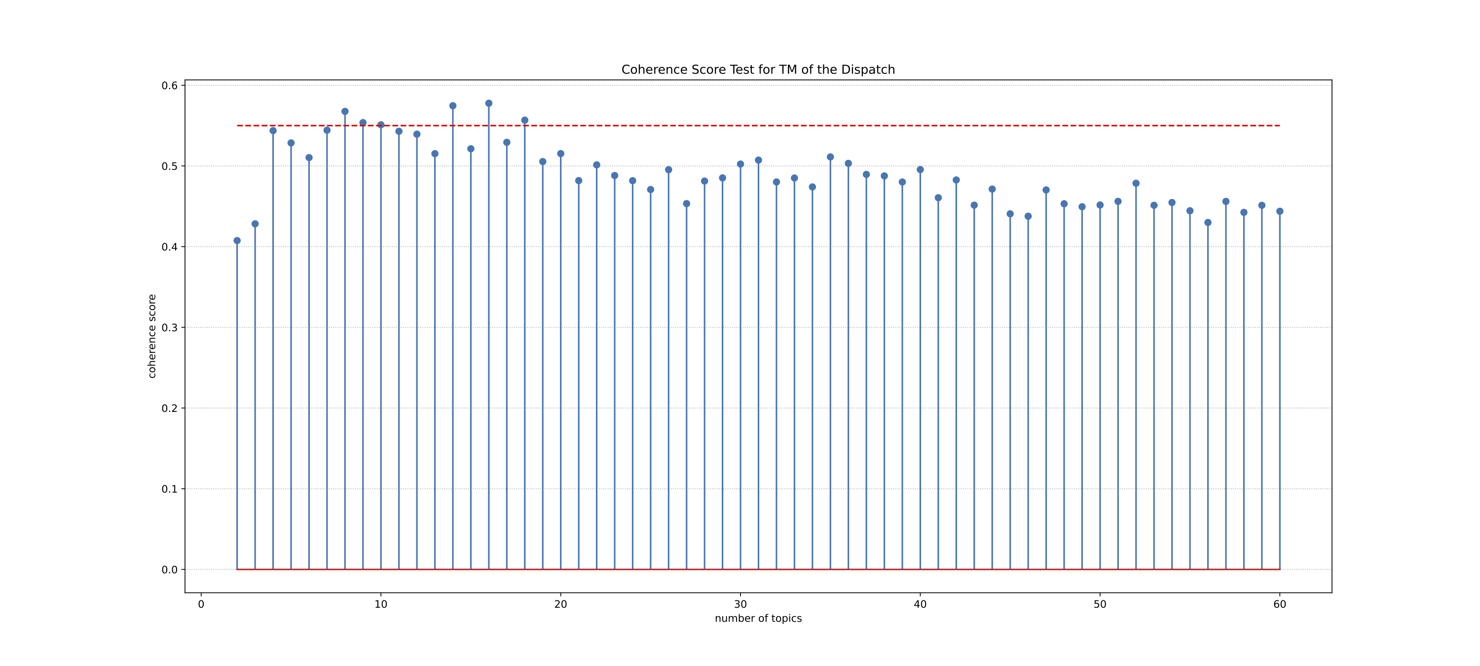
Nonetheless, there is a mathematical way that may help to identify the optimal number of topics. The common practice is to generate several models and calculate coherence score (k) for them all—the number with the highest coherence score is considered optimal (ideally, above 0.55).

The output of the script (for each run with different parameters in # VARIABLES) will generate two files: (1) a TSV file with two columns — the number of topics and corresponding coherence scores; and (2) a graph that visualizes these results. You can reuse the TSV file to graph them differently without rerunning the entire script.

You can get the script from here: topic_modeling_script03.py. Make sure to change dispatchSubfolder if necessary. Keep in mind that running this script with a high number of topics (maxTopic) is likely to take quite a while.

# the script the coherence score test

import io
import pandas

# Gensim
import gensim
import gensim.corpora
from gensim.models import CoherenceModel

import matplotlib.pyplot as plt

import warnings
warnings.filterwarnings("ignore")

from ast import literal_eval # for loading columns with lists

###############################################################################################
# VARIABLES ###################################################################################
###############################################################################################

seedValue = 2023 # this one is needed for reproducability
minTopic   = 2
maxTopic   = 60
fileSuffix = "_years_1860_1864_topics_Min%02d_Max%02d" % (minTopic, maxTopic) 

###############################################################################################
def main():
    print("""
    ######################################################
    Running coherence score test for %d-%d topics
    ::: %s
    random_state value: %d
    ######################################################
    """ % (minTopic, maxTopic, fileSuffix, seedValue))

    # LOAD CORPUS (WE CAN EDIT THIS LIST IN ORDER TO REDUCE THE AMOUNT OF DATA THAT WE ARE LOADING)
    print("="*80)
    print("Loading the corpus")
    dispatchSubfolder = "./Dispatch_Processed_TSV/"
    dispatchFiles = ["Dispatch_1860_tmReady.tsv",  # incomplete
                    "Dispatch_1861_tmReady.tsv",  # The War starts of April 12, 1861
                    "Dispatch_1862_tmReady.tsv",
                    "Dispatch_1863_tmReady.tsv",
                    "Dispatch_1864_tmReady.tsv",
                    #"Dispatch_1865_tmReady.tsv",  # incomplete - The War ends on May 9, 1865
                    ]

    df = pandas.DataFrame()
    for f in dispatchFiles:
        print("\t", f)
        dfTemp = pandas.read_csv(dispatchSubfolder + f, sep="\t", header=0, converters={'textDataLists': literal_eval})
        df = df.append(dfTemp)

    dispatch_light = df
    # drop=True -- use it to avoid creating a new column with the old index values
    dispatch_light = dispatch_light.reset_index(drop=True) 
    dispatch_light["month"] = pandas.to_datetime(dispatch_light["month"], format="%Y-%m")
    dispatch_light["date"] = pandas.to_datetime(dispatch_light["date"], format="%Y-%m-%d")
    print("="*80)

    # PREPARE CORPUS FOR TOPIC MODELING - generate gensim objects: dictionary, corpus, term frequencies (bag of words) 
    print("\tpreparing the corpus")
    dictionary = gensim.corpora.Dictionary(dispatch_light["textDataLists"])
    texts = dispatch_light["textDataLists"]
    corpus = [dictionary.doc2bow(text) for text in texts] # bow == bag of words

    # run optimal number test
    print("\trunning optimal number test...")
    print("="*80)
    optimalTopicsNumber = ["topics\tscore"]

    for num in range(minTopic, maxTopic+1, 1):
        lda_model_temp = gensim.models.LdaModel(corpus=corpus,id2word=dictionary, num_topics=num, random_state=seedValue)
        coherence_model_lda = CoherenceModel(model=lda_model_temp,texts=dispatch_light["textDataLists"],
                                        dictionary=dictionary, coherence='c_v')
        coherence_lda = coherence_model_lda.get_coherence()
        optimalTopicsNumber.append("%d\t%f" % (num, coherence_lda))
        print('\t\tCoherence Score for %02d topics: ' % num, coherence_lda)
        
    print("-"*50)

    # save results
    print("\tSaving results...")
    optimalTopicsNumber = "\n".join(optimalTopicsNumber)
    with open(dispatchSubfolder + "optimal_topic_number_%s.tsv" % fileSuffix, "w", encoding="utf8") as f9:
        f9.write(optimalTopicsNumber)
    print("-"*50)

    # graph results
    scoresData = io.StringIO(optimalTopicsNumber)
    scoresDF = pandas.read_csv(scoresData, sep="\t", header=0)

    plt.rcParams["figure.figsize"] = (20, 9)
    plt.stem(scoresDF['topics'], scoresDF['score'])
    plt.plot([minTopic, maxTopic], [0.55, 0.55], color="red", linestyle="--")

    plt.ylabel("coherence score")
    plt.xlabel("number of topics")
    plt.title("Coherence Score Test for TM of the Dispatch")
    plt.gca().yaxis.grid(linestyle=':')

    plt.savefig(dispatchSubfolder + "optimal_topic_number_%s.pdf" % fileSuffix, dpi=150)
    #plt.show()

###############################################################################################
if __name__ == "__main__":
    main()
###############################################################################################

Below zou can see the visualization of coherence scores generated with the script. (NB: this script takes the longest to run; the time depends on how many sets of topics it needs to check.)

4. Analyzing Topic Modeling Data

The final script in the series analyzes The next script will run a series of analyses on the topic modeling data that we generated in the previous steps. This script produces the results that we now can look into in order to get new insights into our textual data. More specifically, the script generates a series of results:

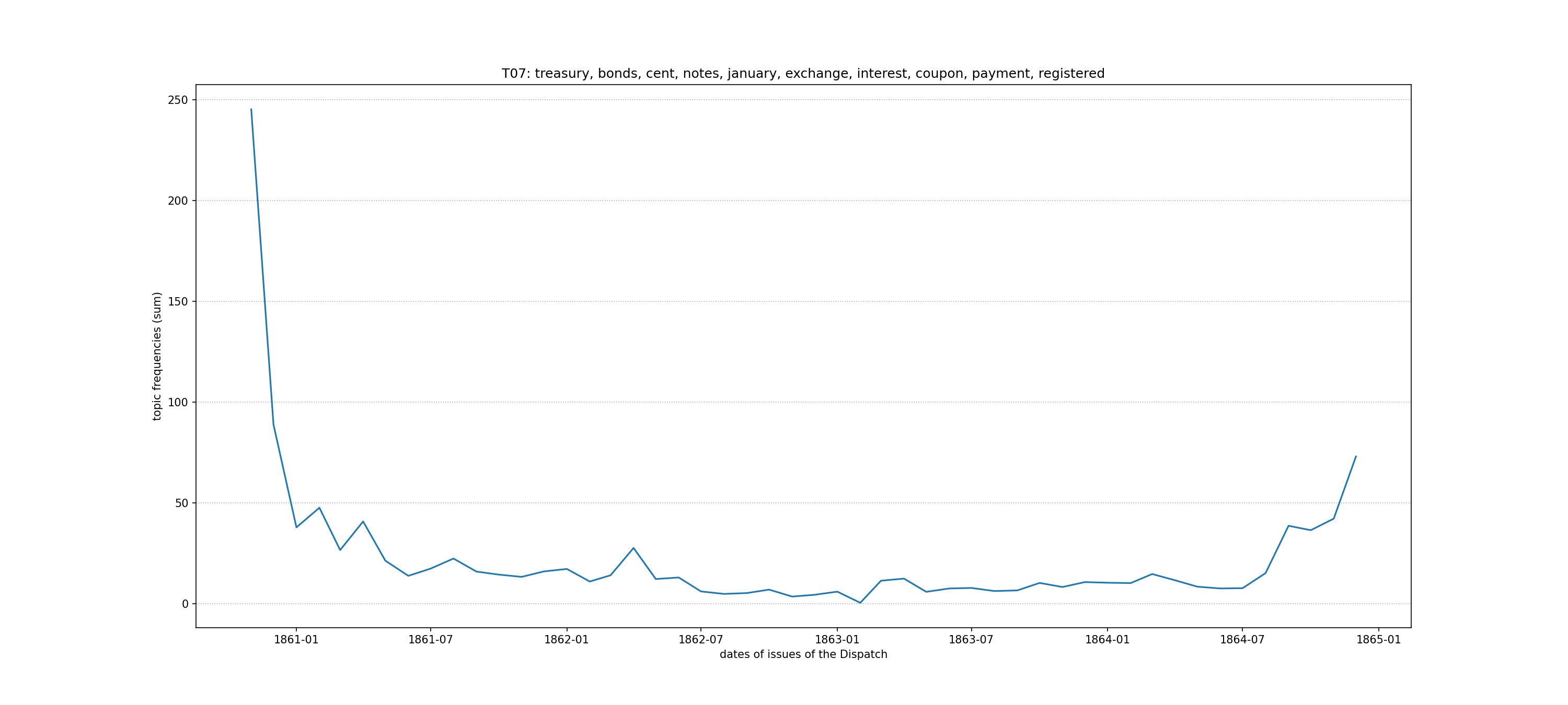
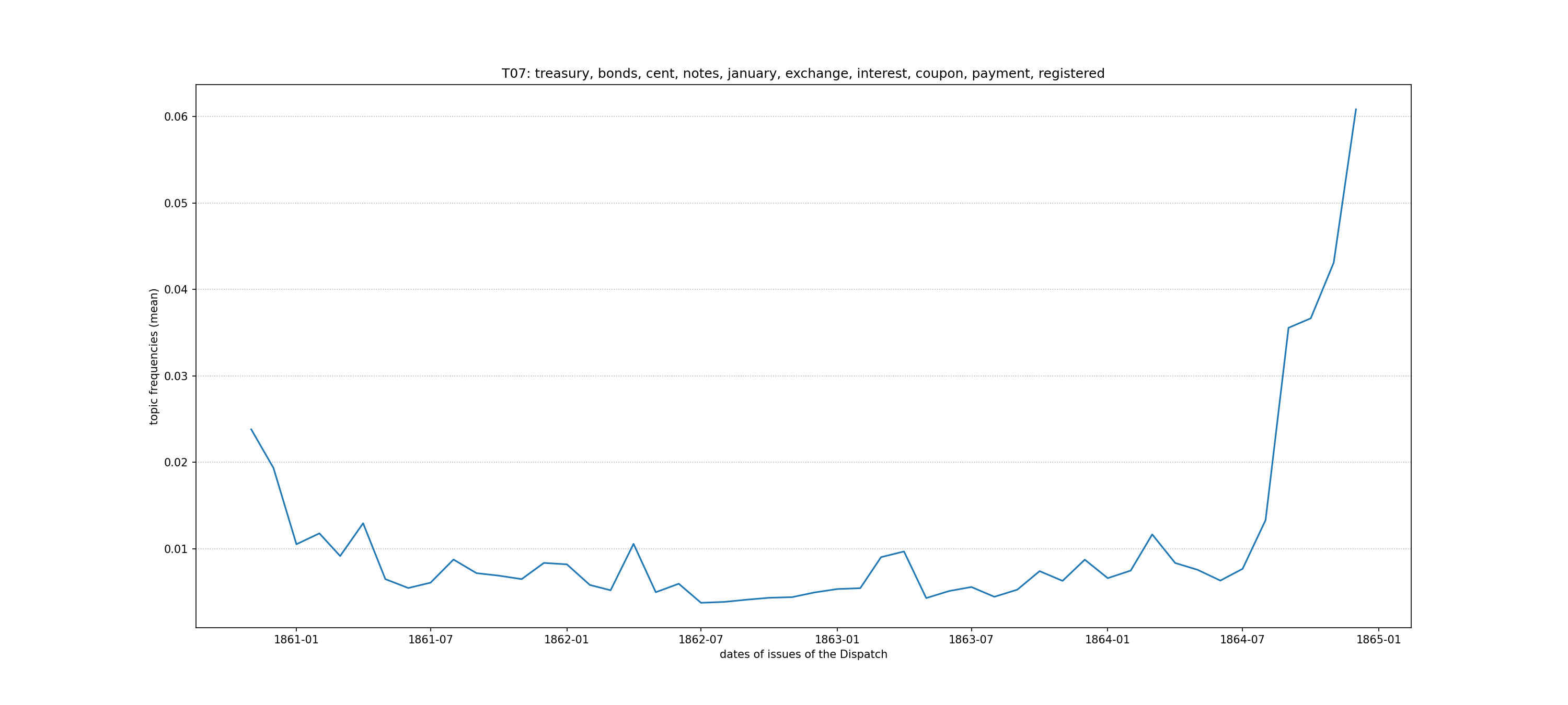
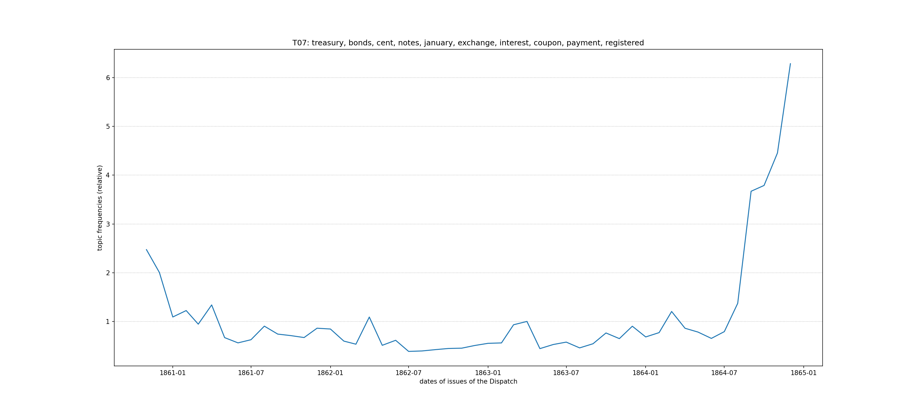
• the script generates a topic explorer (HTML) that allows you to explore topics in more details; by defaults, however, the script does not generate it; in order to generate this visualization, you need to run the main function as main(LDAvisVar=True)
• the script visualizes the distribution of topics over time in three different modes: 1) summed values of each topic over time; 2) average mean of each topic over time; and 3) relative values (percentages) of each topic over time. The script generates two graphs (in PDF and in PNG) per topic per mode (i.e., six graphs per topic in total)
• and finally, the script collects top 100 most representative “articles” per topic and saves them in two different formats for easier exploration afterwards: as a TSV and as a YML files; YML files are more human readable, as we discussed before.

…

# the script runs several analyses of the generated tm data

# the following is to ignore deprecation warnings from pyLDA library; in general, not a good practice as we need to
# write our code in a way that would make it reusable in the future; DeprecationWarning inform us that some element
# of a library in use will stop being usable soonl the annoying thing is the warnings are still printed out...
import warnings
warnings.simplefilter("ignore", FutureWarning, lineno=0)
warnings.filterwarnings("ignore")

import io, json, yaml
import pandas

# Gensim
import gensim
import gensim.corpora
from gensim.models import CoherenceModel

# library for LDA vis
import pyLDAvis
import pyLDAvis.gensim_models as gensimvis

import matplotlib.pyplot as plt

from ast import literal_eval # for loading columns with lists

###############################################################################################
# VARIABLES ###################################################################################
###############################################################################################

seedValue = 2023 # this one is needed for reproducability
numberOfTopics = 40
fileSuffix = "_years_1860_1864_%dtopics" % numberOfTopics
dispatchSubfolder = "./Dispatch_Processed_TSV/"

# files to load
ldaModelFile = "LDA_model__years_1860_1864_%dtopics.lda" % numberOfTopics
topicsNamesFile = "LDA_model__years_1860_1864_%dtopics_TOPICS.json" % numberOfTopics
topicsData = "LDA_model__years_1860_1864_%dtopics_ModeledDataLight.tsv" % numberOfTopics

###############################################################################################
def main(LDAvisVar=False):
    print("""
    ######################################################
    Running analyses based on %d topics
    ::: %s
    random_state value: %d
    ######################################################
    """ % (numberOfTopics, fileSuffix, seedValue))

    # LOAD MODELS and TOPIC NAMES
    print("\tLoading pregenerated topic model: %s" % ldaModelFile)
    ldaModel = gensim.models.LdaModel.load(dispatchSubfolder + ldaModelFile)

    print("\tLoading pregenerated topic names: %s" % topicsNamesFile)
    with open(dispatchSubfolder + topicsNamesFile) as jsonData:
        topicNames = json.load(jsonData)

    # LOAD CORPUS (WE CAN EDIT THIS LIST IN ORDER TO REDUCE THE AMOUNT OF DATA THAT WE ARE LOADING)
    print("="*80)
    print("\tLoading the corpus")
    dispatchFiles = ["Dispatch_1860_tmReady.tsv",  # incomplete
                    "Dispatch_1861_tmReady.tsv",  # The War starts of April 12, 1861
                    "Dispatch_1862_tmReady.tsv",
                    "Dispatch_1863_tmReady.tsv",
                    "Dispatch_1864_tmReady.tsv",
                    #"Dispatch_1865_tmReady.tsv",  # incomplete - The War ends on May 9, 1865
                    ]

    df = pandas.DataFrame()
    for f in dispatchFiles:
        print("\t", f)
        dfTemp = pandas.read_csv(dispatchSubfolder + f, sep="\t", header=0, converters={'textDataLists': literal_eval})
        df = df.append(dfTemp)
    df = df.reset_index(drop=True)
    #print(len(df))

    print("\tLoading the topics data: %s" % topicsData)
    dfTopics = pandas.read_csv(dispatchSubfolder + topicsData, sep="\t", header=0)
    #print(len(dfTopics))

    print("\tMerging tables...")
    dispatch_light = pandas.merge(df, dfTopics, how="left", on="id")
    #print(len(dispatch_light))

    # drop=True -- use it to avoid creating a new column with the old index values
    dispatch_light = dispatch_light.reset_index(drop=True) 
    dispatch_light["month"] = pandas.to_datetime(dispatch_light["month"], format="%Y-%m")
    dispatch_light["date"] = pandas.to_datetime(dispatch_light["date"], format="%Y-%m-%d")
    print("="*80)

    #print(dispatch_light)
    if LDAvisVar:
        print("\tGenerating topics browser (LDAvis)")
        dictionary = gensim.corpora.Dictionary(dispatch_light["textDataLists"])
        texts = dispatch_light["textDataLists"]
        corpus = [dictionary.doc2bow(text) for text in texts]

        modelVis = pyLDAvis.gensim_models.prepare(ldaModel, corpus, dictionary)
        pyLDAvis.save_html(modelVis, dispatchSubfolder + 'tmVis_%s.html' % fileSuffix)
        print("\t\tsaved into: " + 'tmVis_%s.html' % fileSuffix)
    else:
        print("\tTopics browser (LDAvis) was not generated")

    # Generating analyses
    print("\tVisualizing topics over time (grouped by months) - % of a topic per month")
    print("\t\tand: Aggregating most representative articles by topic (into TEXT files)")

    def graphFunc(dataframe, dfType, topic, topicName):
        plt.rcParams["figure.figsize"] = (20, 9)
        plt.plot(dataframe['month'], dataframe[k])
        plt.ylabel("topic frequencies (%s)" % dfType)
        plt.xlabel("dates of issues of the Dispatch")
        plt.title(topic + ": " + topicName)
        plt.gca().yaxis.grid(linestyle=':')
        plt.savefig(dispatchSubfolder + "TopicChronoGraph_%s_%s_%s.pdf" % (fileSuffix, topic, dfType), dpi=150)
        plt.savefig(dispatchSubfolder + "TopicChronoGraph_%s_%s_%s.png" % (fileSuffix, topic, dfType), dpi=150)
        plt.clf()   

    # This will find the average mean for each topic for each month
    topicSumMean = dispatch_light.groupby("month").mean().copy()
    topicSumMean["month"] = topicSumMean.index

    # This will find the sum for each topic for each month
    topicSumSum = dispatch_light.groupby("month").sum().copy()
    topicSumSum["month"] = topicSumSum.index

    # This will find the rel for each topic for each month
    topicSumRel = dispatch_light.groupby("month").sum().copy()
    topicSumRel["total"] = topicSumRel.sum(axis=1) # this calculates the 100% value per month
    for column in topicSumRel:
        topicSumRel[column + "_ABS"] = topicSumRel[column]
        topicSumRel[column] = topicSumRel[column] / topicSumRel["total"] * 100
        topicSumRel[column + "_REL"] = topicSumRel[column]
    topicSumRel["month"] = topicSumRel.index

    # HM, graphs of MEAN are extremely similar to graphs of RELATIVE...
    #topicSumRel.to_csv(dispatchSubfolder + "_TEST.tsv", sep="\t", index=False)
    #print(topicSumRel)

    for k,v in topicNames.items():
        graphFunc(topicSumMean, "mean", k, v) # MEAN GRAPH
        graphFunc(topicSumSum, "sum", k, v) # SUM GRAPH
        graphFunc(topicSumRel, "relative", k, v) # RELATIVE GRAPH

        temp = dispatch_light.sort_values(by=k, ascending=False)
        temp = temp[["id", "text", k]].head(100)
        temp.to_csv(dispatchSubfolder + "TopicSamples_%s_%s.tsv" % (fileSuffix, k), sep="\t", index=False)
        with open(dispatchSubfolder + "TopicSamples_%s_%s.yml" % (fileSuffix, k), "w") as f9:
            yaml.dump(temp.to_dict(orient="records"), f9)


###############################################################################################
if __name__ == "__main__":
    main()
    #main(LDAvisVar=False) # run this if you want to generate the visualization
###############################################################################################

To give you an idea of what the script produces, below are results for Topic 7 (treasury, bonds, cent, notes, january, exchange, interest, coupon, payment, registered). (NB: PDFs are better for publications, as they are in vector graphic, while PNG files are usually better for online use.)

And here is an example (a small part) from a file that includes “articles” that are most representative of the Topic 07 (the complete YML file is here):

- T07: 0.9249956607818604
  id: 1861-08-12_advert_0209
  text: State Bonds for sale.;;; Virginia six per Cent Bonds.;;; Tenn. Six per Cent.
    Bonds.;;; For sale by R. H. Maury & Co. au 2--2w
- T07: 0.8206296563148499
  id: 1862-01-04_article_0192
  text: Stock sale.;;; -- Raleigh and Gaston Railroad stock sale at Raleigh recently
    at 850 per share.
- T07: 0.8078803420066833
  id: 1861-01-18_article_0315
  text: "Sales of Stocks in Richmond, by John A. Lancaster & Son, no. 197 Main\
    \ st, two doors above Farmers' Bank, for the week ending January 17, 1861;;; Virginia\
    \ 6 per cent, Registered Bonds sales $78 \xBD to $80. --;;; Richmond City Bonds,\
    \ sales $87 \xBD;;; Petersburg City Bonds \u2014 no recent sales.;;; Lynchburg\
    \ City Bonds \u2014 no recent sales.;;; Norfolk City Bonds \u2014 no' recent sales.;;;\
    \ Exchange Bank Stock, sales $100.;;; Farmers' Bank Stock, sales 99.;;; Bank of\
    \ Virginia Stock, offered at 68.;;; Bank of the Commonwealth Stock --no sales\
    \ since dividend.;;; Richmond and Danville R. R. Bonds, guaranteed by State of\
    \ Va. No recent sales.;;; Virginia Central R. R. Bonds, guaranteed by State of\

You can get the script from here: topic_modeling_script04.py. Make sure to change dispatchSubfolder if necessary.

This set of scripts can be quite easily adapted for any other data set.

12.5 TF-IDF

TF-IDF is the most common automatic method for identifying keywords in texts. This method is the standard approach for identifying keywords. It was first proposed almost fifty years ago by Spärck Jones (1972); Ramsay (2011), in Chapter 1, offers a detailed humanistic explanation of this approach.

This approach is statistical in its nature and therefore requires a sizable collection of texts for meaningful results. In the case of small collections you are likely to observe that the selection of keywords for the same text change significantly with every new addition to the collection of texts. This is because the method takes into account frequencies of each word and the number of documents in which this word occurs. For example, if your collection includes 10 articles that discuss different aspects of the ʿAbbāsid caliphate, with some focused on politics, some on economics, and some on culture, the word “ʿAbbāsid” will most likely not be included into the list of suggested keywords (since all articles have this term), but words like “politics”, “economics”, and “culture” will be in this list, since they appear only in some articles. If you add ten other articles to your collection—and these will deal, say, with the Ottomans—then the word “ʿAbbāsid” will crawl up in the list of keywords for articles dealing with the ʿAbbasids. In other words, if your collection includes texts on the same broad topic (say, the ʿAbbāsids), the TF-IDF algorithm will assign high keywordness to those terms that point to narrower subjects within the broader subject of the ʿAbbāsids.

In cases when one has to run the topic modeling algorithm on a very large collection of texts, TF-IDF can be used in order to reduce the size of the corpus. That is to say, the corpus is first reduced to the TF-IDF abstractions and then the topic modeling algorithm is applied to these abstractions rather than to the complete initial texts.

TF-IDF abstractions can also be used to identify texts on similar topics across a large corpus of texts. In this approach one would calculate the distance between the vectors of TF-IDF abstractions. This approach mathematically checks whether to what extent two different documents share keywords and to what extent the numeric values of these keywords are similar: the more keywords they share and the more similar the keyword values are, the more similar the texts will be. (More details….)

12.6 Implementation in Jupyter Notebook

Jupyter notebooks is a very popular alternative to regular python scripts. You can try the same code with a jupyter notebook as well. There are some advantages and disadvantages to using them. JN can be quite useful when you are experimenting with some fast operations when you explore your dataset and want to try different things like graphs or data reshaping. If your code requires long time to run, JN maybe rather inconvenient to use.

12.6.1 jupyter notebook

From command line (in your working folder)

# installing
pip install jupyter

# starting
jupyter notebook

Your default browser should open something like this:

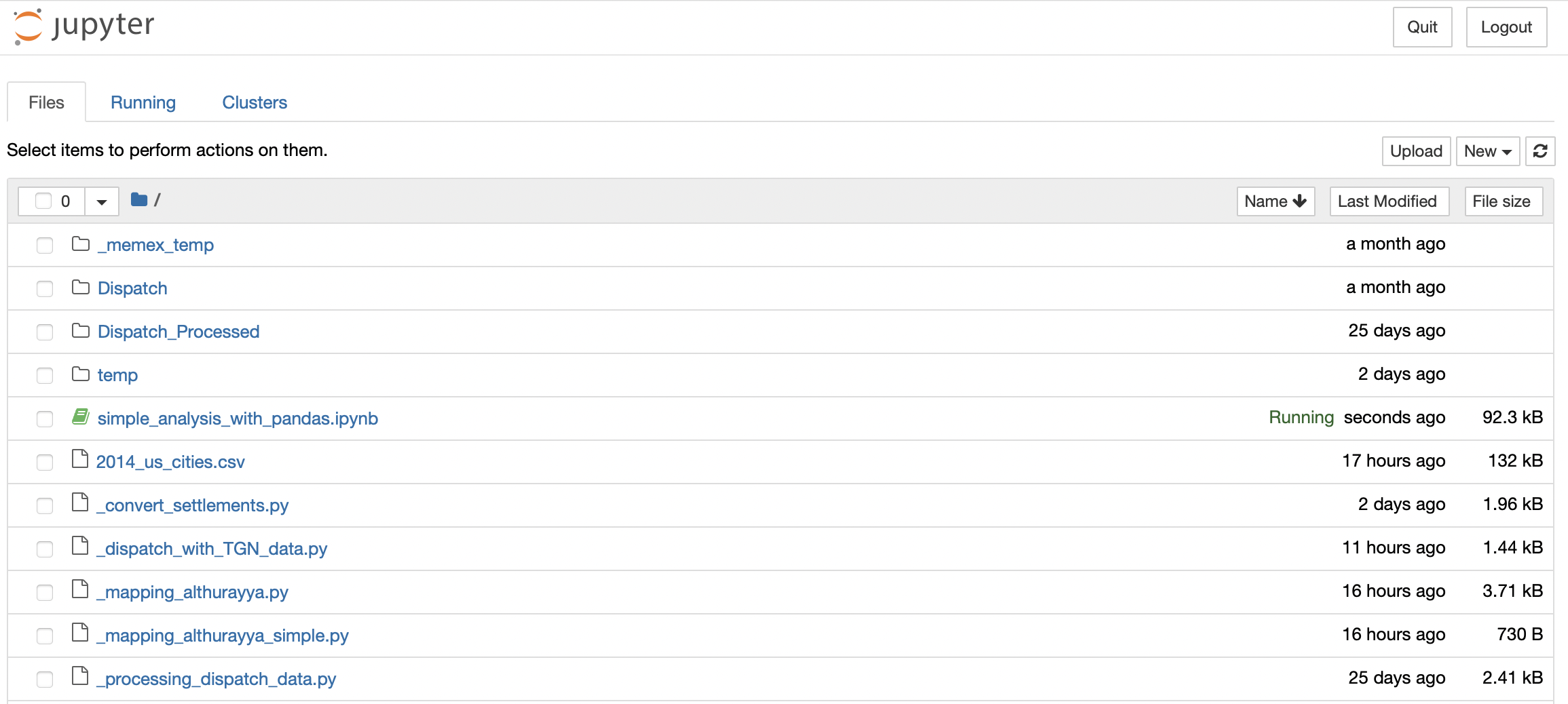
Click on an *.ipynb file to open a notebook.

12.7 Files & Scripts

• Script that converts the Dispatch to TSV files necessary for the Jupyter Notebook; generate these TSV files first, then you can start the Notebook
• TM - Jupyter Notebook
  • For Windows: you will need to deactivate %time in those blocks of code that have it (either delete it, or comment it out with #).

12.8 Homework

• Finish the assigned task;
• Annotate your script (i.e., add comment to every line of code describing what is happenning there);

Submitting homework:

• Homework assignment must be submitted by the beginning of the next class;
• Now, that you know how to use GitHub, you will be submitting your homework pushing it to github:
  • Create a relevant subfolder in your repository and place your HW files there; push them to your GitHub account;
    • Email me the link to your repository with a short message (Something like: I have completed homework for Lesson 3, which is uploaded to my repository … in subfolder L03)

12.9 Solution

No solutions for this lesson…

References

Ramsay, Stephen. 2011. Reading Machines: Toward an Algorithmic Criticism. Topics in the Digital Humanities. Urbana, IL: University of Illinois Press.

Spärck Jones, Karen. 1972. “A Statistical Interpretation of Term Specificity and Its Application in Retrieval.” Journal of Documentation 28 (1): 11–21. https://doi.org/10.1108/eb026526.